| Author: | |
| Website: | |
| Page title: | |
| URL: | |
| Published: | |
| Last revised: | |
| Accessed: |
Matrices can be used to represent linear transformations such as those that occur when two-dimensional or three-dimensional objects on a computer screen are moved, rotated, scaled (resized) or undergo some kind of deformation. Each transformation is represented by a single matrix. Matrices are particularly useful for representing transformations in the field of computer graphics, because each transformation can be represented in a consistent format that is easily represented as a computer data structure. In addition, the transformation represented by a matrix M can be undone by applying the inverse of the matrix. In other words, matrix M -1 reverses the transformation applied by matrix M. We will be looking here at some basic examples of using matrices to represent different kinds of transformations of two-dimensional objects. Let's start with simple reflection.
Imagine a single point A that has the co-ordinates x = 3, y = 4 relative to the origin (0, 0).
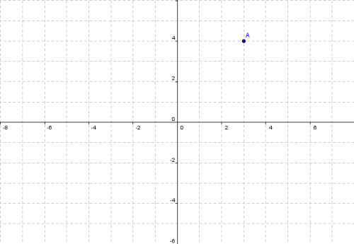
A single point A with xy coordinates (3,4)
Supposing we wish to find the matrix that represents the reflection of any point (x, y) in the x-axis. The transformation involved here is one in which the coordinates of point (x, y) will be transformed from (x, y) to (x, -y). For this to happen, x does not change, but y must be negated. We can therefore achieve the required transformation by multiplying y by minus one (-1). Because we are dealing with a two-dimensional image, all points in the two-dimensional plane are represented by two variables (x and y). The transformations we apply to a point must set values for x and y independently. We will therefore represent our transformation using the two-by-two matrix M:
| M = | a | b | ||
| c | d |
The original position of point A relative to the origin is given by a position vector (x, y) which we can represent using a one-by-two column matrix which we'll call matrix V. By convention, the point created by a transformation is called the image of the original point, and is often given the same label but with the addition of a tick mark (a single apostrophe). Thus A will become A'. The position of point A' relative to the origin after the transformation has been applied is given by the position vector (x, -y), which we can represent using a second one-by-two column matrix which we'll call matrix V '. We can find V ' as follows.
MV = V '
Writing this in matrix form, we get:
| a | b | x | = | x | ||||||
| c | d | y | -y |
When we multiply two matrices, each row in the first matrix is multiplied by each column in the second matrix, so we have:
ax + by = x
cx + dy = -y
In order for the vales of x and y to be transformed independently, elements b and c in matrix M must be zero. We therefore have:
ax = x
dy = -y
So the values of a and d will be one and minus one respectively. We now have:
| 1 | 0 | x | = | x | ||||||
| 0 | -1 | y | -y |
Substituting the original coordinates for point A into vector V 1, we get:
| 1 | 0 | 3 | = | 3 | ||||||
| 0 | -1 | 4 | -4 |
The coordinates for point A' are therefore x = 3, y = -4.
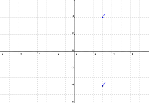
Point A' has xy coordinates (3, -4)
There are a number of simple transformations involving reflection in the coordinate plane that can be achieved using a transformation matrix like the one we saw above. Here are a few examples:
| 1 | 0 | Reflection in the x-axis (see above) | ||
| 0 | -1 |
| -1 | 0 | Reflection in the y-axis | ||
| 0 | 1 |
| 0 | 1 | Reflection in the line y = x | ||
| 1 | 0 |
| 0 | -1 | Reflection in the line y = -x | ||
| -1 | 0 |
These transformations work the same with geometric shapes as they do with a single point. The only difference is that each point in the coordinate plane that defines the shape has a separate vector. Consider the triangle shown below:
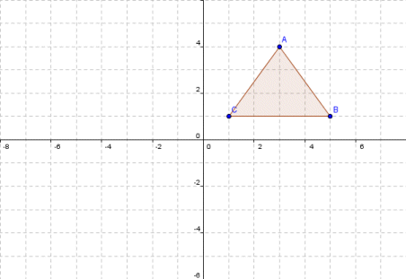
Triangle ABC has xy coordinates of: (3, 4), (5, 1), (1, 1)
Since the points that define the triangle are given by three position vectors, we will require a two-by-three matrix to represent them. Suppose we want to reflect this triangle in the y-axis. The transformation can be achieved as follows:
| -1 | 0 | 3 | 5 | 1 | = | -3 | -5 | -1 | ||||||
| 0 | 1 | 4 | 1 | 1 | 4 | 1 | 1 |
Here is the result of our transformation:
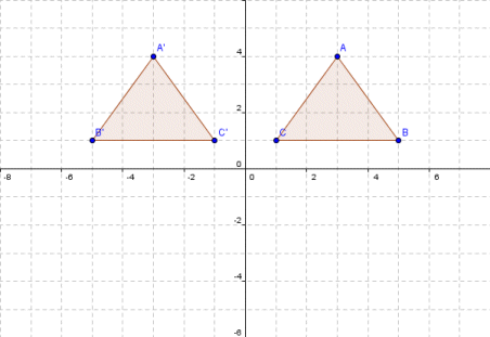
Triangle A'B'C' has xy coordinates of: (-3, 4), (-5, 1), (-1, 1)
We can apply a linear transformation such as reflection to any two-dimensional figure defined by n points in the coordinate plane using the same two-by-two transformation matrix. A two-by-n matrix is used to hold the position vectors for the figure. We saw above the transformation matrix for reflection in the line y = x (which by definition goes through the origin at an angle of forty-five degrees). It is somewhat trickier to find the transformation matrix for a point that must be reflected in a line which, although it goes through the origin, is defined by different values of x and y. As an example, consider the line y = 2x, and a point A with xy coordinates x = 6, y = 3:
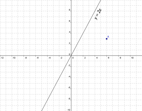
Point A, with xy coordinates of (6, 3) is to be reflected in the line y = 2x
There is a general form for a matrix corresponding to a reflection in the line y = (tan θ ) x, where θ is the angle between the x-axis and the line. The form for the matrix is:
| cos (2θ ) | sin (2θ ) | ||
| sin (2θ ) | -cos (2θ ) |
For our chosen line, y = 2x, θ is given by:
tan (θ ) = 2 ⇒ θ = arctan (2) = 63.43°
If you are wondering how we arrived at this value for θ, remember that the tangent of an angle is given as opposite over adjacent. For a line y = tan (θ ) x, the tangent will be given by Δ y over Δ x (i.e. the slope of the line). For the line y = 2x the slope of the line, and therefore tan (θ ), is two. Once you know the tangent, the angle can be found using the arctan function on your calculator (this is usually labelled tan-1). If we now substitute actual values into our transformation matrix we get:
| cos (2 × 63.43) | sin (2 × 63.43) | = | -0.6 | 0.8 | ||||
| sin (2 × 63.43) | -cos (2 × 63.43) | 0.8 | 0.6 |
Applying this transformation to point A, we get:
| -0.6 | 0.8 | 6 | = | -1.2 | ||||||
| 0.8 | 0.6 | 3 | 6.6 |
The coordinates for point A' are therefore x = -1.2, y = 6.6.
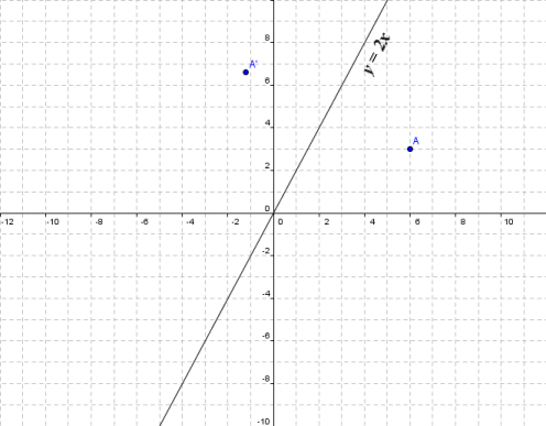
Point A' has xy coordinates (-1.2, 6.6)
Consider the triangle shown below.
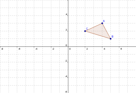
Triangle ABC has xy coordinates: (4,3), (5,1), (2,2)
Suppose that we want to rotate the triangle either clockwise or anti-clockwise about the origin by some arbitrary angle. The matrices required to carry out such transformations are given below.
| cos (θ ) | sin (θ ) | Rotation by θ in a clockwise direction | ||
| -sin (θ ) | cos (θ ) |
| cos (θ ) | -sin (θ ) | Rotation by θ in an anti-clockwise direction | ||
| sin (θ ) | cos (θ ) |
We will put this to the test by rotating our triangle through one hundred and twenty degrees anti-clockwise. The transformation can be achieved as follows:
| cos (120°) | -sin (120°) | 4 | 5 | 2 | = | -0.500 | -0.866 | 4 | 5 | 2 | = | -4.598 | -3.366 | -2.732 | ||||||||||
| sin (120°) | cos (120°) | 3 | 1 | 2 | 0.866 | -0.500 | 3 | 1 | 2 | 1.964 | 3.830 | 0.732 |
Here is the result of the transformation:
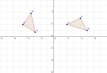
Triangle A'B'C' has xy coordinates: (-4.598, 1.964), (-3.366, 3.830), (-2.732, 0.732)
Scaling (sometimes called dilation) is an operation that changes the size of an object while (usually) maintaining its proportions. It can be achieved very simply by multiplying the position vector matrix by some scalar value. Assume that, after rotating the triangle from the previous example, we then decided to increase its size. We start with the triangle in its new position:
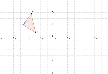
Triangle ABC has xy coordinates: (-4.598, 1.964), (-3.366, 3.830), (-2.732, 0.732)
If we want to increase the magnitude of triangle's position vectors by fifty per cent (50%), we would multiply the vector matrix by one point-five (1.5). The transformation is achieved as follows:
| 1.50 × | -4.598 | -3.366 | -2.732 | = | -6.897 | -5.049 | -4.098 | ||||
| 1.964 | 3.830 | 0.732 | 2.946 | 5.745 | 1.098 |
Here is the result of the transformation:
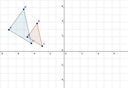
Triangle A'B'C' has xy coordinates: (-6.897, 2.946), (-5.049, 5.745), (-4.098, 1.098)
Note that we could have achieved exactly the same result by multiplying the position vector by the two-by-two matrix that would result from multiplying the two-by-two identity matrix I2 by one point-five:
| 1.5 | 0.0 | -4.598 | -3.366 | -2.732 | = | -6.897 | -5.049 | -4.098 | ||||||
| 0.0 | 1.5 | 1.964 | 3.830 | 0.732 | 2.946 | 5.745 | 1.098 |
This is actually the preferred option in situations where we might want to combine two or more linear transformations in a single two-by-two matrix (we will see how this can be achieved shortly). We can also scale an object in one dimension only - essentially a process of stretching. Suppose for example that we wanted to increase the width of our triangle by a factor of two (2), but leave the height as it is. This linear transformation would be achieved as follows:
| 2.0 | 0.0 | -4.598 | -3.366 | -2.732 | = | -9.196 | -6.732 | -5.464 | ||||||
| 0.0 | 1.0 | 1.964 | 3.830 | 0.732 | 1.964 | 3.830 | 0.732 |
Here is the result of the transformation:
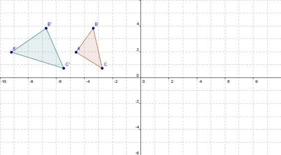
Triangle A'B'C' has xy coordinates: (-9.196, 1.964), (-6.732, 3.830), (-5.464, 0.732)
You may notice that in stretching the triangle in this manner, we have altered the shape of it somewhat. The angles in the triangle A'B'C' are not the same as those in the triangle ABC. From the above, you should be able to work out for yourself the matrix required to stretch a shape by a factor of two in the vertical (as opposed to horizontal) direction. One interesting thing to note here is that the degree to which the area of a figure is increased or decreased by a scaling operation is directly related to the determinant of the transformation matrix. Remembering that a transformation creates an image of the original object, then for a transformation matrix M the following will be true:
area of image = |M| × area of object
In other words, the determinant of a transformation is also a scaling factor for the transformation (note that it is the absolute value of the determinant that is important here, since the determinant may have a negative value if the transformation involves reflection).
The effect of shearing is to distort an object by slanting it in one particular direction. The easiest way to explain the effect is to provide a couple of examples. Consider the following square:
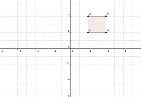
Square ABCD has xy coordinates: (2, 4), (4, 4), (4, 2) , (2, 2)
We can create a shear effect in the horizontal direction from left to right by multiplying the value of x in each position vector by a value that is proportional to y. This has the effect that the points at the top of the figure are pushed further to the right than the points at the bottom of the figure. Supposing we apply the following transformation:
| 1.0 | 1.5 | 2 | 4 | 4 | 2 | = | 8 | 10 | 7 | 5 | ||||||
| 0.0 | 1.0 | 4 | 4 | 2 | 2 | 4 | 4 | 2 | 2 |
The effect of this transformation is to add one-and-a-half times the value of y to x for every position vector of the figure. Obviously, as y increases, the increase in x will become greater. We can see the effect of applying this transformation below. The result is a parallelogram, and the distortion has taken place parallel to the x-axis.
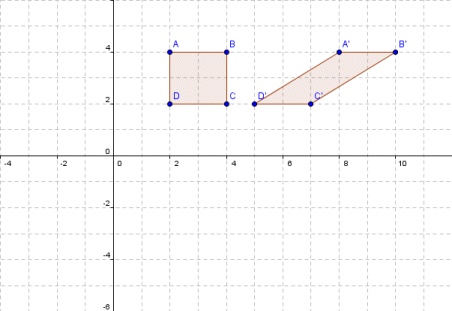
The shearing transformation produces a parallelogram
Note that for a transformation of this type (i.e. a horizontal shear), any points lying on the x-axis will not change position, since the value of y will be zero. Let's see what happens when we apply a similar transformation in the vertical direction. Here is a triangle with one side parallel to the y-axis:
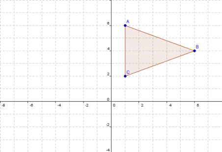
Triangle ABC has xy coordinates: (1, 6), (6, 4), (1, 2)
This time we will create a shear effect in the vertical direction from bottom to top by multiplying the value of y in each position vector by a value that is proportional to x. This will have the effect that the points at the right of the figure are pushed further in the upwards direction than the points at the left of the figure. Let's apply the following transformation:
| 1 | 0 | 1 | 6 | 1 | = | 1 | 6 | 1 | ||||||
| 1 | 1 | 6 | 4 | 2 | 7 | 10 | 3 |
The effect of this transformation is to add one times the value of x to y for every position vector of the figure. Obviously, as x increases, the increase in y will become greater. We can see the effect of applying this transformation below. The result is a triangle that is a highly-distorted version of the original, with the distortion taking place parallel to the y-axis.
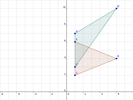
A vertical shearing transformation applied to a triangle
Note that for a transformation of this type (i.e. a vertical shear), any points lying on the y-axis will not change position, since the value of x will be zero. The general form for each type of transformation is given as:
| x' | = | 1 | k | x | x increases by ky in the horizontal direction | ||||||
| y' | 0 | 1 | y |
| x' | = | 1 | 0 | x | y increases by kx in the vertical direction | ||||||
| y' | k | 1 | y |
The process of combining transformations is known as composition. Two or more linear transformations can be combined with relative ease using matrix multiplication. For example, let's assume we have two matrices, A and B, that represent two different linear transformations. Assuming that we have a position vector matrix X1, We can apply these transformations one after the other (first A, then B), as follows:
X2 = AX1
X3 = BX2
The same end result can be achieved by applying the transformation that is created by multiplying matrices A and B together. Note, however, that the order in which the matrices must be multiplied is the opposite of the order in which they should be applied. Thus, in order to achieve the same end result as we did previously we would have:
X3 = BA (X1)
Consider the following triangle:
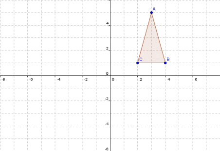
Triangle ABC has xy coordinates: (3, 5), (4, 1), (2, 1)
Supposing we want to rotate the triangle clockwise through ninety degrees, and then reflect it in the y-axis. The two transformations matrices would be:
| cos (90°) | sin (90°) | = | 0 | 1 | Rotation by 90° in a clockwise direction | ||||
| -sin (90°) | cos (90°) | -1 | 0 |
| -1 | 0 | Reflection in the y-axis | ||
| 0 | 1 |
Applying these transformations separately, we get:
| 0 | 1 | 3 | 4 | 2 | = | 5 | 1 | 1 | ||||||
| -1 | 0 | 5 | 1 | 1 | -3 | -4 | -2 |
| -1 | 0 | 5 | 1 | 1 | = | -5 | -1 | -1 | ||||||
| 0 | 1 | -3 | -4 | -2 | -3 | -4 | -2 |
Here is the first transformation:
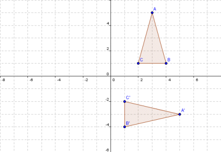
Triangle ABC is rotated ninety degrees to become triangle A'B'C'
Here is the second transformation:
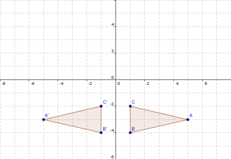
Triangle ABC is reflected in the y-axis to become triangle A'B'C'
We could create a transformation matrix that combines these operations by multiplying the two individual transformation matrices together as follows:
| -1 | 0 | 0 | 1 | = | 0 | -1 | ||||||
| 0 | 1 | -1 | 0 | -1 | 0 |
Note that we multiply the matrices in the opposite order to that in which we want them to be applied. If we now multiply the resulting transformation matrix by the position vector matrix of our original triangle we get:
| 0 | -1 | 3 | 4 | 2 | = | -5 | -1 | -1 | ||||||
| -1 | 0 | 5 | 1 | 1 | -3 | -4 | -2 |
If you refer back to the results we got when we carried out the rotation and reflection transformations separately, you will see that the final x and y coordinates for each point are identical.
Any transformation that is not achieved by multiplying a position vector matrix by a two-by-two transformation matrix is non-linear (or at least, not strictly linear). One such transformation is called translation, which simply means that the object is moved by a given distance in a particular direction (i.e. along a given vector). For example, consider the following triangle:
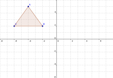
Triangle ABC has xy coordinates: (-4, 5), (-2, 2), (-6, 2)
Now supposing we want to move the triangle eight units to the right and six units down. We can achieve this by using matrix addition, as follows:
| -4 | -2 | -6 | + | 8 | 8 | 8 | = | 4 | 6 | 2 | ||||||
| 5 | 2 | 2 | -6 | -6 | -6 | -1 | -4 | -4 |
Here is the result of the transformation:
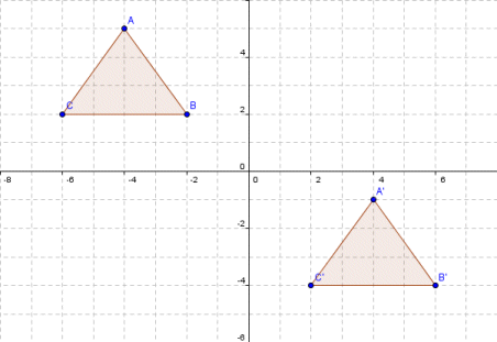
Triangle A'B'C' has xy coordinates: (4, -1), (6, -4), (2, -4)
Note that the transformation matrix for a translation must be the same size (i.e. have the same number of rows and columns) as the vector matrix of the figure it transforms, since this is a pre-requisite for matrix addition. Note that both linear and non-linear transformations can be applied to a two-dimensional figure. Normally, the two types of operation are carried out using separate matrices, but under certain circumstances they may be combined in a single matrix. A transformation that involves both linear and non-linear operations is called an affine transformation.