| Author: | |
| Website: | |
| Page title: | |
| URL: | |
| Published: | |
| Last revised: | |
| Accessed: |
We are often asked to find the derivative of an expression in which one variable (the dependent variable, usually called y) is expressed as a function of another variable (the independent variable, usually called x). In mathematical terms, we can write this as y = ƒ(x). This will not always be the case, however. Sometimes we are faced with situations in which it is not possible to express y in terms of x (or vice versa), but where we can express both x and y in terms of a third variable, which by convention we usually call t (probably because it is often used to represent time). We call this third variable a parameter.
A function that has this third variable (or parameter) is called a parametric function. The process of differentiating a parametric function is called parametric differentiation. As you might expect, differentiating a parametric function is somewhat more complicated than differentiating a function that only has two variables, but it is possible. Before we actually look at how to differentiate parametric functions, however, it might help to look at an example of a parametric function and see what its graph (which we call a parametric curve) looks like.
The first thing to note is that a parametric function is actually written as two separate functions. Let's start by thinking about the equation of a circle having a radius of one unit centred at the origin (i.e. the unit circle). We would normally write this equation in terms of x and y as:
x 2 + y 2 = 1
What we have here is effectively an implicit function - i.e. a function in which the dependent variable is not isolated on one side of the equation. Alternatively, we can rewrite the equation for the unit circle in parametric terms. This, as we have already said, actually involves two separate (though related) functions. Each of these functions will take a range of values that enable them to define the coordinates of all of the points on the circumference of the circle. The first function defines the x coordinates of all the points that make up the circle. We can write this function as:
x(t) = cos (t) or just x = cos (t)
In this first function, x is the dependent variable while t is the independent variable. The second function defines the y coordinates of the points that make up the circle. We can write this function as:
y(t) = sin (t) or just y = sin (t)
In this second function, y is the dependent variable, and t is again the independent variable. We therefore have two dependent variables, x and y, both of whose values depend on the value of a single parameter, t. If we don't put a limit on the range of values that t is allowed to take, both x and y will cycle endlessly through the same range of values. If we want to trace out the unit circle once only (and assuming that t is expressed in radians), we should restrict the range of values t can take to a lower limit of zero and an upper limit of 2π. Our complete parametric function for the unit circle can therefore be written as:
x = cos (t), y = sin (t) for 0 ≤ t ≤ 2π
Here is the graph of the function:
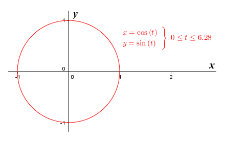
The graph of the parametric function x = cos (t), y = sin (t) for 0 ≤ t ≤ 2π
One of the most obvious differences between parametric (and to some extent implicit) functions and explicit functions (in which x and y are the independent and dependent variables respectively) is that the horizontal direction of a curve created by graphing an explicit function cannot change, whereas for a parametric (or implicit) function, it can. This allows for some very interesting possibilities, but it also means that parametric curves have a distinct direction of motion with respect to t. In the case of the parametric function x = cos (t), y = sin (t) for 0 ≤ t ≤ 2π, plotting the graph of the function traces out the unit circle in the anti-clockwise direction, starting from xy coordinates (1, 0).
To further illustrate this, let's look at the graph of another parametric function. This time we'll consider the function x = t 2 + t, y = 2t - 1. Note that for now, we will not specify any limits on the value of t. Here is the graph of the function:
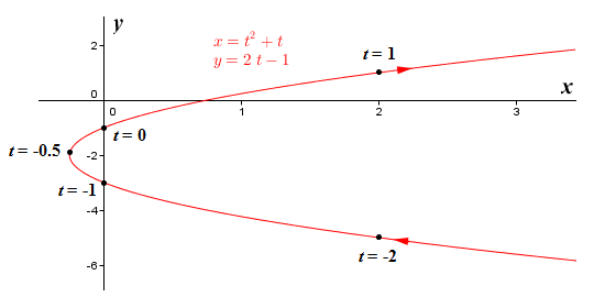
The graph of the parametric function x = t 2 + t, y = 2t - 1
Note the arrows on the curve. They indicate the curve's direction of motion, i.e. the direction in which the plot will "grow" as the value of t increases. The curve changes its horizontal direction when the value of t reaches minus zero-point-five (-0.5). This is the value of t for which the function returns the lowest possible value of x, which is minus zero-point two-five (-0.25). The curve itself is a parabola that opens to the right. Because no limits are imposed on the values that may be taken by t, both arms of the parabola will extend to infinity in the positive horizontal direction. Note however that the direction of movement will be negative in the lower arm and the positive in the upper arm. If we limit the range of values taken by t to a minimum value of minus one (-1) and a maximum value of one (1), we get the following parametric curve:
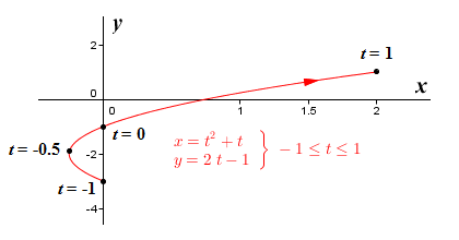
The graph of the parametric function x = t 2 + t, y = 2t – 1 for -1 ≤ t ≤ 1
This curve is identical to the curve we had before we imposed limits on the value of t, except that the lower arm is truncated at the y axis, and the upper arm extends only as far as x = 2. Depending on the precise nature of the parametric function and the limits imposed upon it, plotting the graph of a parametric function will sometimes result in a curve that is traced out repeatedly. To visualise the kind of thing we are talking about, think about a parametric function that models the movement of a pendulum bob. Parametric functions can also be used to model much more complex behaviours. For that reason, they are often used in fields such as physics to describe the motion of a particle, or the trajectory of a projectile.
Now that we have established in general terms what a parametric function is, and what a typical parametric curve looks like, we will turn to the question of how to differentiate a parametric function. This will obviously be somewhat more involved than differentiating explicit functions defined in terms of x and y only. After all, we now have three variables to think about (including the parameter t), and a different kind of function - one that is actually two separate, though closely related, functions. Yet, despite these differences, the derivative that we are looking for is still the slope of a graph plotted using x and y coordinates. In other words, we are still looking for dy/dx.
It would certainly be easier if we could treat y as if it were a function of x. Actually, if you think about it, even though it may not be possible to express y as a function of x in the way we have previously, we can see from examining the graph of a parametric function that y does indeed vary as x varies. This means, that y can still be considered to be a function of x, even if we can't define that function. Let's state this formally:
y = ƒ(x)
Don't forget though that y is also an explicit function of t, which we'll identify as g(t):
y = g(t)
Although we don't know what the function ƒ(x) actually does, this is something we don't need to worry about. We already know the most important thing about x, which is that it is an explicit function of t. We'll identify this function as h(t):
x = h(t)
You should by now have realised that ƒ(x) is a composite function, for which the inner function is h(t). We can therefore express the relationships between the functions we have identified as follows:
y = g(t) = ƒ(x) = ƒ(h(t))
Remember that if we want to differentiate a composite function, we need to use the chain rule. The chain rule tells us that in order to find the derivative of the composite of two functions, we need to multiply the derivative of the outer function by the derivative of the inner function. So, differentiating with respect to t, we can now write the following:
g′(t) = ƒ′(h(t)) h′(t)
Hopefully you can see that this is equivalent to writing:
g′(t) = ƒ′(x) h′(t)
Unfortunately, the notation we have been using has necessarily involved the use of somewhat arbitrary function names, which could become a little confusing as we attempt to move forward. In order to clarify things, let's rewrite the derivative using Liebniz's notation (which you should already be reasonably familiar with, if you have been working through the pages in this section in order). Here is the revised version:
| dy | = | dy | × | dx |
| dt | dx | dt |
Bearing in mind that what we are ultimately looking for is dy/dx, we need to rearrange things a little:
| dy | = |
|
||
| dx |
|
Or alternatively:
| dy | = | dy | × | dt |
| dx | dt | dx |
Let's have a look at an example. We'll find the derivative of the parametric function x = t 2 + t, y = 2t - 1, which we saw earlier. First we apply the appropriate rules of differentiation to find the derivative of y = 2t - 1 with respect to t:
| dy | = 2 |
| dt |
Now we find the derivative of x = t 2 - 1 with respect to t:
| dx | = 2t + 1 |
| dt |
Remember that we need to find dt/dx. This is simply the reciprocal of dx/dt:
| dt | = | 1 |
| dx | 2t + 1 |
So the derivative of x = t 2 + t, y = 2t - 1 is given by:
| dt | = | 2 |
| dx | 2t + 1 |
That was all relatively straightforward, but how do we now use this result to find the slope (i.e. the derivative) of our parametric function at a given point, which is after all the purpose of differentiation? First of all, how do we define the point at which we want to find the slope? Well, let's assume for the moment that we want to find the slope for a given value of t. This seems reasonable, since t is effectively the independent variable here and often represents time. Suppose we want to find the slope m of the curve when t = 1. Plugging this value for t into the derivative function, we get:
| dy | = | 2 | = | 2 |
| dx | 2 + 1 | 3 |
Assuming we want to draw the tangent representing the slope of the curve for t = 1, we need to find the x and y coordinates that correspond to this value of t:
x = t 2 + t = 2
y = 2t - 1 = 1
Remember that the equation of a line is y = mx + b, where m is the slope of the line and b is the y intercept. Since we have the slope, and the x and y coordinates for a point on the line, we can find the intercept:
b = y - mx = 1 - ( 2/3 × 2) = -1/3
So the equation that describes our tangent line will be:
y = 2/3 x - 1/3
The illustration below shows the graph of the function together with the tangent line to the curve at point (2, 1).
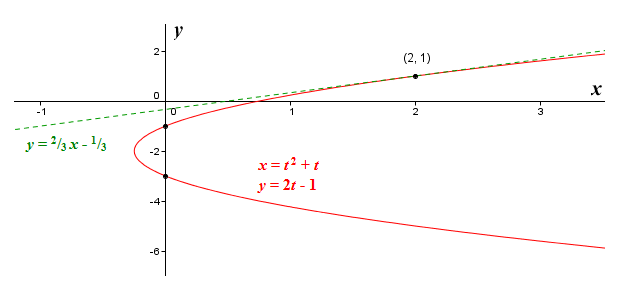
The graph of x = t 2 + t, y = 2t – 1 and the tangent to the curve at (2, 1)
Let's work through another example. This time we'll find the derivative of the parametric function x = cos (2t), y = sin (3t). This will introduce a complication that might already have occurred to you, given the fact that parametric functions can produce curves that behave in ways that we have not previously encountered, but we'll come to that in due course. First, we will find the derivative of y = sin (3t) with respect to t (remember, we need to use the chain rule):
| dy | = 3 cos (3t) |
| dt |
Now we find the derivative of x = cos (2t) with respect to t:
| dx | = -2 sin (2t) |
| dt |
Again, we need to find dt/dx, which is the reciprocal of dx/dt:
| dt | = | 1 |
| dx | -2 sin (2t) |
So the derivative of x = cos (2t), y = sin (3t) is given by:
| dy | = - | 3 | × | cos (3t) |
| dx | 2 | sin (2t) |
Before we go any further, let's see what the curve produced by this function looks like.
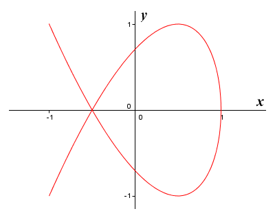
The graph of x = cos (2t), y = sin (3t)
This function is interesting for a couple of reasons. Remember what we said earlier - that some functions trace the same curve out repeatedly. This is a perfect example of such a function. As t increases, the function traces out the curve you can see here repeatedly, first in one direction and then the other (which is why there are no arrows indicating direction of movement). Each complete cycle requires an interval of 2π (i.e. t will increase by 2π during each cycle). The other especially interesting thing to note here is that the top and bottom halves of the curve are mirror images of one another. In fact, the arms of the curve cross one another at point (-0.5, 0). If we are asked to find the slope of the function at this point, there could be two possible answers (although there will of course only be one correct answer for a specific value of t).
The curve is traced out in one direction in an interval of π - i.e. t will increase by π as the curve is traced out completely in one direction only. The slope of the curve at any point will be the same, regardless of the direction of movement, so the derivative we obtain when the value of t is set to some fraction of π will be the same as the derivative for values of t set to that fraction plus some multiple of π. Let's find a couple of tangents to this curve. First, we'll find the derivative when t = 1/6 π. Plugging this value for t into the derivative function, we get:
| dy | = - | 3 | × | cos (1/2 π) | = 0 |
| dx | 2 | sin (1/3 π) |
This would indicate that we are looking at a horizontal tangent. Now we'll find the x and y coordinates that correspond to this value of t:
x = cos (2t) = cos (1/3 π) = 0.5
y = sin (3t) = sin (1/2 π) = 1
Now we can plug the values we have obtained into the equation of the line once again to obtain the y intercept:
b = y - mx = 1 - (0 × 0.5) = 1
So the equation that describes our tangent line will be:
y = 0x + 1 = 1
This is the equation of a horizontal line that intercepts the y axis at y = 1. You can probably already see that this line will indeed be a tangent to the curve at point (0.5, 1). For the sake of completeness, we present once more the graph of x = cos (2t), y = sin (3t) together with the horizontal tangent to the local maximum at x = 0.5.
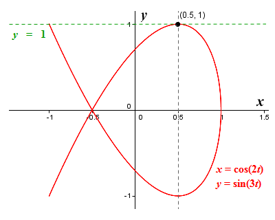
The graph of x = cos (2t), y = sin (3t) and the tangent to the curve at (0.5, 1)
Now, we'll find the derivative when t = 1/4 π. Plugging this value for t into the derivative function, we get:
| dy | = - | 3 | × | cos (3/4 π) | = - | -2.121 | = 1.061 |
| dx | 2 | sin (1/2 π) | 2 |
Next, we'll find the x and y coordinates that correspond to this value of t:
x = cos (2t) = cos (1/2 π) = 0
y = sin (3t) = sin (3/4 π) = 0.707
Plug these values into the equation of the line to obtain the y intercept:
b = y - mx = 0.707 - (1.061 × 0) = 0.707
The equation that describes our tangent line will be:
y = 1.061x + 0.707
Here is the graph of x = cos (2t), y = sin (3t), this time showing the tangent to point (0, 0.707).
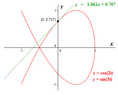
The graph of x = cos (2t), y = sin (3t) and the tangent to the curve at (0, 0.707)
We can also find the higher derivatives of a parametric function. Higher derivatives can offer give us useful information about a function. The second derivative, for example, can tell us about the concavity of a curve at a particular point and, providing certain conditions are met, can also tell us whether a local extremum is a local maximum or a local minimum. Let's take a look at how we can find the second derivative of a parametric function. As you might expect, this is slightly more complicated than finding the higher derivatives of an explicit function that only has two variables.
By now, you should know that the second derivative of a function (parametric or otherwise) is the derivative of the derivative of the function. First, let's think about how we find the first derivative of a parametric function. Remember that we are essentially dealing with two functions. One function gives us the value of x in terms of t, while the other function gives us the value of y in terms of t. It is relatively easy to obtain the derivatives of these functions separately, which we can then plug into the formula for the derivative of a parametric function. Here is the formula once more:
| dy | = |
|
||
| dx |
|
or:
| dy | = | dy | × | dt |
| dx | dt | dx |
What we need to find now is a formula for the second derivative of the function, i.e. the derivative of the derivative, which in Liebniz's notation is written as d 2y/dx 2. If you have read the page "Basic Rules of Differentiation", you might remember that, for some function ƒ(x), we express the derivative of the function as:
| dy | = | d | (ƒ(x)) |
| dx | dx |
The notation d/dx essentially just tells us that we are taking the derivative of some function with respect to x (just to clear up any possible confusion, the notation dy/dx tells us explicitly that we are taking the derivative of y as a function of x). So, given that the derivative of a function is essentially just another function, we can write the second derivative as follows:
| d 2y | = | d | ( | dy | ) |
| dx 2 | dx | dx |
If we expand this, we get:
| d 2y | = | d | ( |
|
) | ||
| dx 2 | dx |
|
Now, if we rearrange this somewhat, we get:
| d 2y | = | d | ( | dy | ) | dt |
| dx 2 | dt | dx | dx |
And that, essentially, is the formula for the second derivative. Not exactly intuitive, but it works. What we've done, effectively, is to apply the chain rule again, this time to the first derivative, in order to get the second derivative. To demonstrate that our formula works, let's work through a couple of examples. We'll start by finding the second derivative for the parametric function x = t 5 – 4t 3, y = t 2. Obviously, we will need to find the first derivative before we do anything else. Apply the appropriate rules of differentiation to find the derivative of y = t 2 with respect to t:
| dy | = 2t |
| dt |
Now find the derivative of x = t 5 - 4t 3 with respect to t:
| dx | = 5t 4 - 12t 2 |
| dt |
Remember that we need to find dt/dx. This is simply the reciprocal of dx/dt:
| dt | = | 1 |
| dx | 5t 4 - 12t 2 |
So the first derivative of x = t 5 – 4t 3, y = t 2 is given by:
| dy | = | 2t |
| dx | 5t 4 - 12t 2 |
Simplifying this, we get:
| dy | = | 2 |
| dx | 5t 3 - 12t |
Now to find the second derivative, which we have established is given by:
| d 2y | = | d | ( | dy | ) | dt |
| dx 2 | dt | dx | dx |
So:
| d 2y | = | d | ( | 2 | ) | × | 1 |
| dx 2 | dt | 5t 3 - 12t | 5t 4 - 12t 2 |
First, we'll differentiate dy/dx with respect to t. We'll need to use the quotient rule here, which you might remember tells us that the derivative of the quotient of two functions is equal to the product of the denominator and the derivative of the numerator, minus the product of the numerator and the derivative of the denominator, all over the denominator squared. So, we have:
| d | ( | 2 | ) | = | 24 - 30t 2 |
| dt | 5t 3 - 12t | (5t 3 - 12t) 2 |
We now need to multiply this result by dt/dx:
| d 2y | = | 24 - 30t 2 | × | 1 | = | 24 - 30t 2 |
| dt 2 | 5t 3 - 12t | 5t 4 - 12t 2 | (5t 4 - 12t 2)(5t 3 - 12t) 2 |
Simplifying gives us:
| d 2y | = | 24 - 30t 2 | = | 24 - 30t 2 |
| dt 2 | t (5t 3 - 12t)(5t 3 - 12t) 2 | t (5t 3 - 12t) 3 |
And that's it, we have the second derivative.
Let's work through one more example problem. Suppose we want to find the second derivative of the parametric function x = t 3 + 3t 2, y = t 4 - 8t 2. As before, we'll start by finding the first derivative. Differentiating y = t 4 - 8t 2 with respect to t gives us:
| dy | = 4t 3 - 16t |
| dt |
And differentiating x = t 3 + 3t 2 with respect to t gives us:
| dx | = 3t 2 + 6t |
| dt |
We find dt/dx by taking the reciprocal of dx/dt:
| dt | = | 1 |
| dx | 3t 2 + 6t |
So the first derivative of x = t 3 + 3t 2, y = t 4 - 8t 2 is given by:
| dy | = | 4t 3 - 16t |
| dx | 3t 2 + 6t |
We can simplify this as follows:
| dy | = | 4t (t 2 - 4) |
| dx | 3t (t + 2) |
| dy | = | 4t (t - 2)(t + 2) |
| dx | 3t (t + 2) |
| dy | = | 4 (t - 2) |
| dx | 3 |
Just to remind you, the formula for the second derivative is:
| d 2y | = | d | ( | dy | ) | dt |
| dx 2 | dt | dx | dx |
Plugging the results we have obtained into this formula, we get:
| d 2y | = | d | ( | 4 (t - 2) | ) | 1 |
| dx 2 | dt | 3 | 3t (t + 2) |
We will use the quotient rule to differentiate dy/dx with respect to t:
| d | ( | 4 (t - 2) | ) | = | 4 |
| dt | 3 | 3 |
We multiply this result by dt/dx:
| d 2y | = | 4 | × | 1 | = | 4 |
| dt 2 | 3 | 3t (t + 2) | 9t (t + 2) |
And once again, we have found the second derivative.