| Author: | |
| Website: | |
| Page title: | |
| URL: | |
| Published: | |
| Last revised: | |
| Accessed: |
Both analogue and digital signals are used in telecommunications systems, although there has been a steady migration from analogue to digital transmission across a range of industry sectors, most notably in the areas of telephony services and television broadcasting. Radio broadcasting is also gradually moving towards digital transmission, albeit at a somewhat slower pace.
The Public Switched Telephone Network (PSTS) is today largely digital, although for the first hundred years or so of its existence the voice-grade telephony services it offered employed end-to-end analogue signal transmission over copper loops, earning it the acronym "POTS" (Plain old Telephone Service).
The introduction of digital carrier systems in the telephone network dates back to the early 1960s, and gained momentum in the 1980s when very large scale integration (VLSI) made it possible to build sophisticated application-specific integrated circuits (ASICs), and more powerful general purpose microprocessors, that simplified the design and manufacture of digital signal processing equipment.
Today, the only part of the telephone system that is still mostly analogue is the local loop, sometimes known as the subscriber loop or the last mile - the physical link between the customer's home or business premises and the local telephone exchange. Even here, digital technologies such as ISDN, DSL and FTTx have made significant inroads. British Telecom are tentatively planning to shut down the PSTN in the UK by 2025, after which all telephone voice traffic will be carried on its national fibre broadband network using Voice over IP (VoIP) technology.
Until the late 1990s, virtually all television broadcast signals, whether received via a roof-mounted aerial, a cable, or a satellite dish, were analogue. By the end of the first decade of the new millennium, much of the existing analogue television broadcasting technology in Western Europe had been replaced by digital broadcasting technology, reducing broadcasting costs and providing greatly improved picture and sound quality to consumers. At the time of writing, the digital switchover in most European countries is either complete or nearing completion.
Satellite TV led the way in the transition from analogue to digital, mainly because the necessary changes on the transmission side only involved the earth station equipment, and because end users were already familiar with the use of a set-top box. Many European countries had terminated analogue satellite broadcasts by the year 2000. The last country in Europe to switch off analogue satellite transmissions was Germany, in 2012.
Countries in Europe that have now completed the transition from analogue to digital include Austria, Denmark, France, Greece, Ireland, Italy, Luxembourg (the first country to complete the switchover, in 2006), Norway, Spain, and the United Kingdom. Several other European countries have terminated satellite and terrestrial analogue broadcasts but retain some analogue cable services, including Belgium, Germany, Portugal and Sweden. In the Netherlands, major cable TV provider Ziggo began phasing out analogue services in 2018, and expects to complete the process by the End of 2020.
The switch to digital radio broadcasting has been much slower for a number of reasons, despite the fact that audience numbers generally have been holding their own and even increasing in recent years with the proliferation of Internet radio stations and the emergence of new community, local, and national radio broadcast services. In the UK, the number of listeners accessing radio digitally only exceeded the number listening to analogue radio as recently as May 2018.
Digital Audio Broadcasting (DAB) has been around for many years now, but the uptake has been slow. Problems with audio quality and reception during the early stages of development didn't help. There were also some technical issues, mainly due to the complexity of the circuitry required to decode signals. The resulting high power consumption meant that DAB receivers were bulkier than their analogue counterparts and had a much shorter battery life, although improvements to circuitry design have since levelled the playing field somewhat.
AM radio broadcasting has certainly been in decline for many years, not helped by the fact that the propagation of AM radio signals increases at night due to a reduction in the effects of ionisation in the upper atmosphere, which means it can cause interference with other stations using the same frequencies. The AM band is also quite noisy, and subject to interference from a number of sources including, vehicle ignition systems and power lines.
FM radio is a different story. At the time of writing, although the sale of radio receivers overall is slowly declining, analogue radios are still significantly out-selling digital radios (although analogue receivers sold since 2013 have also supported the new DAB+ standard). A full switchover from analogue to digital radio broadcasting will no doubt happen eventually (Norway became the first country to end national radio broadcasts on FM in 2017) but no date has currently been set for the UK. The criteria for making that decision are:
Once these three criteria have been met, the UK Government is obligated to announce a date for the switchover from analogue to digital within two years.
From the foregoing, it would seem that we are heading for a predominantly digital future. Data communications is by its very nature inherently digital, and the phasing out of analogue telephony and broadcasting services is already in the final stages. This does not mean that we can afford to forget about how analogue systems work. There will probably always be niche applications that use analogue signalling for reasons of cost and convenience, and the fundamental principles are still highly relevant. Indeed, the passband transmission of digital data is essentially a form of digital-to-analogue conversion!
The word analogue (or analog, if you live in North America) means something that is similar or comparable to something else in some respect. It comes from the Greek word logos, meaning ratio. A sketch or line drawing of a person or object could be considered to be an analogue - in this case a two-dimensional representation - of that person or object. In a hospital environment, the visual output of a heart monitor could be described as an analogue of a patient's heart function.
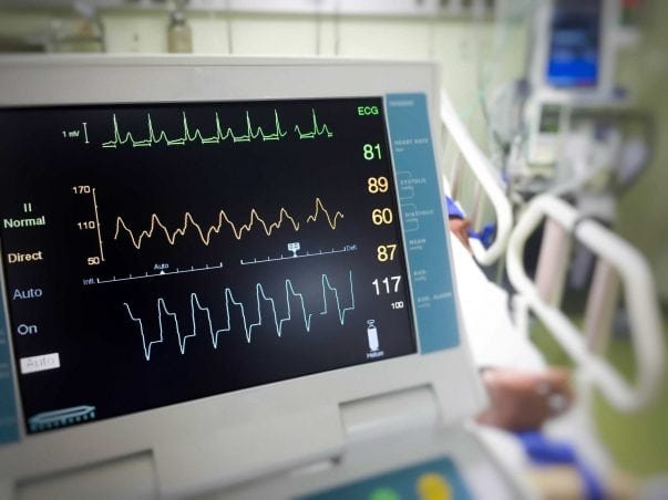
A heart monitor outputs an analogue representation of heart function
An analogue signal, in the context of telecommunications, is any continuous, time-varying signal that is representative of some other time-varying quantity. The voltage waveform on an analogue telephone line, for example, is an analogue of the soundwaves produced by a person speaking into a telephone mouthpiece. In a broader sense, any continuous time-varying signal - a sinusoidal waveform, for example - may also be regarded as an analogue signal.
A typical analogue signal
Analogue signals can carry either analogue or digital information - though not usually both at the same time. The telephone voice signals that are sent and received over the local loop of the Public Switched Telephone Network (PSTN) are still, for the most part, analogue signals. The voice signal is transmitted over a twisted-pair copper wire link as a time-varying AC voltage superimposed on the DC current (supplied by the phone company) that powers the telephone circuitry. The waveform of the AC voltage mimics the waveform of the soundwaves created by the human voice.
The signals generated by AM radio transmitters are also analogue in nature, but the original baseband audio signal has been used to modulate the amplitude of a high-frequency sine wave carrier. The frequency of the carrier wave does not change, but its amplitude is varied in direct proportion to the varying power level in the modulating signal. The same principle applies to the signals generated by FM radio, except that here, the frequency of the carrier wave is varied in proportion to the way that the power level varies in the modulating signal.
Baseband analogue signals can be used to modulate a high-frequency carrier wave
Regardless of the type of modulation used, the modulated high-frequency carrier wave is still an analogue signal, both on account of the fact that it remains a sinusoidal waveform, and because some aspect of it (either amplitude or frequency) is constantly varying in accordance with the variations in signal power of the baseband analogue signal used to modulate it. The modulation process essentially transposes the original analogue signal to a much higher frequency so that it can be transmitted wirelessly.
The interesting thing to note here is that baseband digital signals can also be used to modulate a high-frequency carrier wave, allowing digital information to be transmitted through the airwaves at radio frequencies. Is the resulting signal digital or analogue? On the one hand, the transmitted signal can be considered to be an analogue signal because it is a sinusoidal and thus constantly varying waveform. On the other hand, the fluctuations in amplitude or frequency will be discrete, because they represent digital values.
In the article "Bits, Bauds and Bandwidth", we look at digital signalling methods that use square wave pulses to represent binary ones and zeros. We point out, however, that those pulses are created by combining a sine wave at the fundamental frequency of the digital signalling scheme with successive odd harmonics in order to approximate a square wave. So in essence, even a digital signal consisting of nominally square wave pulses is generated using analogue components.
In fact, all of the signals we use to transmit information, whether the information itself is analogue or digital in nature, can be described as analogue signals. Even the pulses of light that represent binary ones and zeros on an optical fibre - though they are of incredibly short duration - possess both wavelength and frequency. There are no instantaneous transitions from one energy level to another in nature, except perhaps at the quantum level. To all intents and purposes then, the universe we live in is predominantly analogue.
In order to avoid confusion, however, we will reserve the use of the term analogue signal for signals that actually carry analogue information. If a signal carries digital information, we will call it a digital signal. There is in fact one very important difference between these two kinds of signal, which is that even a small fluctuation in an analogue signal may convey some kind of information. This means that any distortion of the signal caused by or noise or interference has the potential to corrupt the information being carried. Digital signals represent discrete values using significant variations in the amplitude, frequency or phase of a carrier wave, and are thus far less sensitive to interference and noise.
The information that human beings acquire from the environment through their five basic senses (sight, hearing, smell, taste and touch) is analogue in nature. The instruments that we use to measure and record such information are usually electronic devices of one kind or another - microphones, digital cameras, temperature sensors, and so on. These devices often produce a digital output, but before that can happen, the real-world inputs must be converted into an electrical signal. A device that converts one form of energy into another is called a transducer.
We use transducers every time we make or receive a telephone call. The microphone in a telephone handset is a transducer, because it turns the acoustical energy produced by the human voice (i.e. soundwaves) into electrical energy (a constantly varying voltage). Up until the 1980s, these microphones consisted of carbon granules sandwiched between two thin metal plates. Sound waves cause the outer plate (or diaphragm) to vibrate, creating small changes in the density of the carbon granules by compressing and uncompressing them.
The line voltage supplied by the telephone company is applied across the microphone when the handset is lifted. The changes in the density of the carbon granules caused by someone speaking into the microphone alters the electrical resistance of the microphone, allowing more or less current to flow through it. Since the resistance of the telephone wire itself does not change, and since voltage varies in direct proportion to current for a given resistance, the changes in the current flowing through the microphone can be seen as changes in the voltage across the telephone line.
A carbon microphone converts soundwaves to a variable voltage
The current passing through the microphone varies in frequency and amplitude in response to the soundwaves arriving at the diaphragm, effectively producing an AC voice signal that rides on top of the DC current. The waveform of this AC signal is an analogue of the soundwaves that are responsible for creating it.
When somebody (the caller) makes a phone call to another person (the call recipient) who is connected to the same local telephone exchange, the switch at the exchange simply establishes an analogue circuit between the two telephones. Otherwise, the analogue voice signal will be digitised for transmission over one or more digital trunk lines, and converted back to an analogue signal at the call recipient's local exchange.
Either way, the voice signal arriving at the call recipient's handset must be converted back into soundwaves in order for them to hear the voice of the caller. A transducer of some kind must be used to convert the electrical energy in the signal back into acoustical energy. In a telephone handset, this takes the form of a small built-in speaker. Because the incoming voice signal is relatively weak, it goes through an amplifier that forms part of the telephone's circuitry before being sent to the speaker.
Several different kinds of speaker have been used in telephone handsets. The diagram below shows the basic construction of a speaker that employs a magnetic diaphragm to produce sound.
A speaker in the handset converts electrical signals to soundwaves
The construction of the microphone is relatively simple. A permanent magnet is mounted inside a non-magnetic housing. Two magnetic pole pieces are attached to the magnet and project towards the front of the housing, effectively creating an arrangement similar to a U-shaped horseshoe magnet. A flexible magnetic diaphragm is mounted across the end of the microphone housing opposite the permanent magnet, with a small gap between it and the ends of the pole pieces.
Each pole piece is arranged so that the end nearest to the diaphragm has the same polarity as the permanent magnet pole to which it is attached, and each pole piece has a wire coil wound on to it. The diaphragm is attracted by the permanent magnet, and when at rest it is held close to the ends of the pole pieces.
When the amplified AC electrical signal passes through the coils, it turns the pole pieces into electromagnets that alternately attract and repel the diaphragm as the polarity of the signal changes, thus causing the diaphragm to vibrate. The vibrations will have the same frequency and amplitude as the voice signals, resulting in localised changes in air pressure that produce soundwaves, effectively reproducing the caller's voice.
The quality of telephone voice reproduction is not perfect because some of the frequencies in the human voice are filtered out in order to simplify the design and implementation of the telephone system, but in most cases it is good enough to enable the call recipient to recognise the voice of the caller (and vice versa).
A more detailed examination of the circuitry used in telephones is beyond the scope of this article. As you have probably realised, however, since voice signals are carried in both directions on the same wire pair simultaneously, some additional circuitry is required to prevent the signals from interfering with each other. In addition, a small portion of the microphone output is sent to the speaker as a means of assuring the user that the telephone is actually working (this is known as audio feedback or acoustic feedback).
A digital signal carries information as a series of binary digits, each of which can take one of two values (zero or one). The precise nature of the digital signal will depend on the kind of encoding scheme used, which is in turn largely dependent on the nature of the communication channel over which the signal is sent. As a general rule of thumb, the signals sent over short distances using guided media such as twisted pair copper cables or optical fibres will usually be baseband signals. For longer distances, and for most types of wireless transmission, passband signalling is used.
We'll look at baseband signalling - sometimes called line coding - first. Baseband signalling is used on virtually all fixed links in local area networks. Various methods can be used to implement baseband signalling. The first method we will look at is a simple line coding scheme in which square wave pulses are used to represent the binary ones and zeros. The presence of a pulse represents a binary one, while the absence of a pulse represents a binary zero. The illustration below illustrates this kind of scenario.
A simple digital signal
In the scheme illustrated above, a binary one is represented by the presence of a voltage on the line (in this case five volts), while a binary zero is represented by the absence of a voltage. The signal thus has just two logic states. In order to decode the signal, the receiver must be able to detect which of these two states the signal is in during each bit interval. This means that the receiver must sample the signal once during each bit interval.
You may occasionally come across the terms mark and space in connection with digital signals, whereby the term mark is used to refer to a binary one, and space refers to a binary zero. These terms originated back in the early days of telegraphy, with the telegraph system developed by the American inventor Samuel Morse (1791-1872). Morse's original design used an electromagnet that caused a pen to move across a moving strip of paper and make a mark whenever current passed through it. When the current was turned off again, the pen would be retracted, leaving a space on the paper.
Baseband digital signals are characterised as discontinuous, because they can only take one of a small number of discrete values at any given time. However, in the real world, signals are never discontinuous. They cannot instantaneously transition from one state to another. As shown in the diagram, the voltage requires time to change from zero volts to five volts or vice versa. During the transition from low to high (the rise time) or from high to low (the fall time) the receiver will not be able to sample the signal reliably because the voltage will be rapidly changing.
Because the receiver must sample the signal in the middle of each bit-time, it needs to know the exact time at which each bit starts, and the duration of each bit. That is only possible if the receiver's clock is synchronised with that of the transmitter. The transmitter will usually send a special sequence of bits called a preamble to let the receiver know that it is about to transmit some data, and to enable the receiver to synchronise its clock with that of the transmitter.
It might be possible for the receiver to re-adjust its clock whenever a transition from high to low (or vice versa) signals the start of a new bit-time, but the clocks can still become out of sync when a long sequence of ones or zeros is transmitted. If the clocks drift apart by even a tiny amount during each bit-time, the receiver will end up sampling the signal too early or too late, detecting either more bits or fewer bits than have actually been sent. This only has to happen once, and all of the data that follows is rendered meaningless.
At relatively low data rates, or for asynchronous transmissions involving only a few bits or bytes of data, the receiver's internal clock signal is usually sufficient to maintain synchronisation with the transmitter long enough to sample the incoming bits in each block of data received at (or close to) the centre of each bit-time. For higher data rates where bit-times become shorter, or for synchronous data transfers involving thousands of bits of information, the receiver's internal clock cannot be relied upon to remain synchronised with the transmitter, and a more reliable timing mechanism is required.
One option is for the transmitter to send a separate timing signal to enable the receiver to maintain synchronisation with the transmitter at all times. The clock signal consists of an alternating digital signal such as a square wave generated by the transmitter and sent over a separate link between the transmitter and the receiver. Clock ticks at the receiver are triggered by either the rising or falling edge (or in some cases both edges) of the incoming signal, allowing the receiver to sample the data stream in the middle of each bit-time.
A separate clock signal provides synchronisation between transmitter and receiver
Unfortunately, the use of a separate clock signal is not a particularly practical solution in most cases because it significantly increases bandwidth usage and makes the transmission system both more difficult and more expensive to design and implement.
There are other serious problems with the simple digital signal we saw above. For example, if we are using the absence of a voltage to signify a binary zero, how does the receiver know when the line is idle? A more serious problem is that the signal is unipolar - only a positive voltage is used - resulting in a significant DC (direct current) component. This can lead to signal distortion at the receiver, and results in energy being lost on the transmission line due to the wires being heated up by the direct current.
We can mitigate the problem of DC current to a great extent by using a bipolar encoding scheme in which binary one is represented by a positive voltage and binary zero is represented by a negative voltage. We can also embed the required timing signal in the data itself by encoding the data in such a way that there is a guaranteed transition from high to low - or from low to high - during each bit-time.
One such encoding scheme, called Manchester encoding (see below), is used in 10BASE-T Ethernet networks. The scheme guarantees a transition in the middle of each bit-time that serves as both a clocking mechanism and as a method of encoding the data. A low-to-high transition represents a binary one, while a high-to-low transition represents a binary zero. This type of encoding is known as bi-phase digital encoding because a transition from one to zero or vice versa is represented by a 180° shift in the signal's phase.
Manchester encoding is a bi-phase, bi-polar digital encoding scheme
Encoding schemes like Manchester encoding are said to be self-clocking, and have no net DC component (there are both positive and negative voltage components of equal duration, during each bit-time). More complex encoding schemes are used for the more recent Ethernet standards. For example, the PAM5 signalling scheme illustrated below is used for the 100BASE-T2 and 1000BASE-T standards (we will be examining how the various line coding schemes work in more detail in another article).
A 5-level pulse-amplitude modulation (PAM5) digital encoding scheme
PAM5 encoding has five signalling symbols, each represented by a different voltage level. Four symbols are used to represent some combination of two binary digits. The fifth symbol is used for forward error correction. Thanks to some very sophisticated electronics, data can be transmitted in both directions simultaneously on a single wire pair, with each wire pair capable of a gross bit rate of 250 Mbps. For Gigabit Ethernet over twisted pair (1000BASE-T), all four wire pairs in the Ethernet cable are used, giving a total gross bit rate of 1000 Mbps.
If we want to send digital information wirelessly we need to use a passband signalling scheme. This involves using the (relatively) low-frequency baseband signal carrying the original digital data stream to modulate a radio frequency (RF) carrier wave. In essence, the same modulation techniques can be used for transposing baseband digital signals onto a high-frequency carrier wave as are used for baseband analogue signals. The main difference is that the modulation will produce discrete changes in the amplitude, frequency or phase of the carrier wave rather than continuous changes.
Amplitude modulation (AM) schemes modulate the amplitude of an RF carrier wave using a digital signal. The carrier will be switched between two or more different power levels, with each power level representing one or more binary digits. In the simplest form of amplitude modulation, individual bits are represented by the presence or absence of the carrier wave, depending on whether a binary one or a binary zero is being transmitted. This method is sometimes called on-off keying.
On-off keying - a simple form of amplitude modulation
Frequency shift keying (FSK), as the name suggests, involves the frequency of an RF carrier wave being shifted up or down to represent either a binary value or a specific bit pattern. In the simplest form of frequency shift keying, binary ones and zeros are represented by shifting the carrier frequency above or below the centre frequency, with the frequencies used being equidistant from the centre frequency. In most schemes, the higher frequency represents a binary one, and the lower frequency represents a binary zero, as shown in the diagram below.
In a simple frequency-shift keying scheme, the signal shifts between two frequencies
Phase-shift keying (PSK) is a modulation method in which the phase of a high-frequency carrier wave is phase-shifted between two or more phase values in order to represent different binary values or bit sequences. The simplest form of phase-shift keying is a form of bi-phase modulation in which the phase of the signal is shifted through π radians (180 degrees) to signal a change in the logic state of the data (i.e. from one to zero, or vice versa). When the receiver detects a phase change in the signal, it must examine the value of the last bit received in order to determine the value of the bit currently being received.
Simple bi-phase frequency-shift keying
Most of the passband signalling schemes used for the transmission of digital signals are far more complex than the simple schemes shown above, but we will be covering them in more detail elsewhere. You should by now have a reasonable grasp of the underlying principles behind each type of modulation, and be able to see the difference between passband and baseband digital signalling.
We have seen how real world analogue information is converted to an analogue signal, in the form of a constantly varying current or voltage, by a transducer. However, when analogue data must be processed by a computer, or stored on some form of digital media, or transmitted over a digital data link, it must first be converted into a digital format - a process known as digitisation.
Digital data represents information using a finite number of discrete values. Whereas analogue data can represent every possible value of the real world entity it is modelling, digital data can only approximate those values within predefined parameters. Suppose we want to represent a temperature measured in degrees Celsius using an unsigned 8-bit binary number. We'll assume that the can vary between 0 and 100 degrees, and that our temperature sensor is an analogue device that outputs a voltage of between 0.0 volts (0 degrees) and 10.0 volts (100 degrees).
An unsigned 8-bit binary number can represent any decimal integer value between 0 and 255. A temperature of 0 degrees Celsius will therefore be represented by 0, and a temperature of 100 degrees will be represented by 255. For argument's sake, let's suppose our sensor is reading a temperature of exactly 63.8 degrees Celsius. The actual voltage reading will be 6.38 volts. What digital value will represent that temperature?
To find the 8-bit binary value that represents this temperature reading, we need to divide the highest value in our digital scale by 100 to determine what value on that scale represents one degree Celsius. We can then multiply that value by the voltage reading returned by our sensor, and then multiply the result by 10 to obtain a digital value for our temperature reading. Here is the calculation:
255 ÷ 100 = 2.55
2.55 × 6.38 × 10 = 162.69
You will notice that we do not get an integer result. The 8-bit number we will use to represent that result, however, must be one of the integer values in our digital scale. We therefore take the nearest value, which is 163. Clearly, there are limitations to the accuracy with which we can represent a real-world value using a digital scale. We could of course increase the precision of the scale by using more bits. If we used 16 bits to represent our temperature scale, we would have 65,536 values to choose from (0 - 65535), and our calculation would be as follows:
65,535 ÷ 100 = 65.355
65.355 × 6.38 × 10 = 41,811.33
Again, we need to take the nearest number in our digital scale, which is 41,811, but the precision of our temperature representation will be greatly improved. The down side is that in order to store that value we need twice as much memory. More importantly from the point of view of sending the data over a data link is that there will be twice as many bits to send, which will take twice as long.
In order to make the most efficient use of the available bandwidth, we need to know how good our representation needs to be in order for it to be good enough for a given application. But before we can answer that question properly, we need to know a little bit more about how the analogue-to-digital conversion process works. There are actually two distinctly separate processes involved - sampling and quantisation. We'll look at sampling first.
The sampling process involves repeatedly measuring the amplitude of the analogue signal we want to digitise. If the signal represents audio or video information, it will vary constantly over time, and in a manner that is difficult to predict. We will need to take a large number of samples during a given time interval in order to create an accurate digital representation of the signal. The frequency with which we take those samples is called the sample rate, and is measured in hertz.
Consider for a moment what happens when you listen to streamed music on your computer or smartphone. The original music was probably recorded in a studio using analogue recording equipment. At some point it was digitised and saved to a digital storage medium such as an optical disc or a computer hard drive, and it is this digitised version that is sent to your device. Your computer or smartphone must interpret the digital data in order to turn it into an analogue signal. A transducer then converts the analogue signal into acoustical energy, which you hear as music.
How many samples do we need to take from the original (analogue) recording in order to be able to recreate the sound on your device to an acceptable standard? The sample rate must be high enough for the device to recreate the sound its original form - or at least close enough to its original form to be deemed fit for purpose. The Swedish born US scientist Harry Nyquist (1889-1976) discovered that the original analogue signal can be reconstructed using a low-pass filter (we'll talk more about that later), so long as the sampling frequency is at least twice as high as the highest frequency in the analogue signal.
The sampling rate must be at least twice that of the highest frequency
The range of frequencies that the human ear can detect is generally accepted to be between 20 Hz and 20,000 Hz (20 kHz). The highest frequency we need to record in order to achieve an acceptable listening experience from a musical recording is thus 20 kHz. According to Nyquist, in order to digitise our analogue recording, we need to sample it with a frequency of 40 kHz. That's a sample rate of 40,000 samples per second! For largely historical reasons that we won't go into here, an audio CD can actually represent frequencies of up to 22.5 kHz, which requires a sampling rate of 44.1 kHz.
Analogue telephone lines use baseband frequencies of between 300 Hz and 3.4 kHz. When a telephone voice signal is digitised, it is convenient to assume a highest frequency of 4 kHz, which requires a sampling rate of 8,000 samples per second. Each sample is encoded using eight bits, so a digital telephone link has a bit-rate of 64,000 bits per second, or 64 kbps (this is the bit rate used for ISDN voice channels).
When we are representing discrete values such as alphanumeric characters and symbols, the number of bits we need to represent each character or symbol will depend on how many characters or symbols we need to represent. In the ASCII character set, for example, there are 128 characters, including alphanumeric characters, punctuation symbols, special characters and control codes. This allows an ASCII character to be represented by a unique sequence of just seven bits, although ASCII characters are usually stored as eight-bit bytes. Character sets like Unicode use up to four bytes to store characters, enabling over one million unique characters and symbols to be stored.
In order to store information about a constantly changing signal waveform however, we are faced with a dilemma. At any given time, the amplitude of the signal can have any one of an infinite number of possible values. Once we have sampled the signal and acquired a value, we have to give that value a number - a process known as quantisation. The number we use will be one of a set of discrete values, the size of which will be limited by the number of bits we have available to represent each value.
If we have a large set of discrete values to choose from, our quantisation will represent the sample values accurately, but the number of bits we need to represent each sample will increase, which increases the amount of digital data we need to send. If, on the other hand, we limit the number of bits per sample to reduce bandwidth usage, the end-user device may not be able to reconstruct the analogue signal in is original form.
The numerical difference between the sampled value and the value assigned to it in by the quantisation process is known as quantisation error. We cannot avoid quantisation error, because unless we use a very large number of bits to represent each sample - which is not really a practical option - there will always be a difference, however small, between the sample value and the digital value it is assigned.
The real question is, how good is good enough? How many distinct levels do we need to use in order to accurately represent an analogue signal? Because that will dictate how many bits we must use to store the value of each sample. Let's assume that we are sampling an analogue signal that varies between -1 volt and +1 volt. If we use a 4-bit one's complement binary number to represent each level, we will have fifteen levels available (-7 to +7) to represent the voltage of the AC waveform. Each level will represent a specific voltage, as follows:
| Level | Binary representation | Voltage |
|---|---|---|
| -7 | 1000 | -1.00 v |
| -6 | 1001 | -0.85 v |
| -5 | 1010 | -0.71 v |
| -4 | 1011 | -0.57 v |
| -3 | 1100 | -0.43 v |
| -2 | 1101 | -0.29 v |
| -1 | 1110 | -0.14 v |
| 0 | 0000 | 0.00 v |
| 1 | 0001 | +0.14 v |
| 2 | 0010 | +0.29 v |
| 3 | 0011 | +0.43 v |
| 4 | 0100 | +0.57 v |
| 5 | 0101 | +0.71 v |
| 6 | 0110 | +0.85 v |
| 7 | 0111 | +1.00 v |
How good is our representation going to be? Let's look again at the waveform we used above to illustrate the sampling process, and assume that it represents an AC waveform that varies between -1 and +1 volts.
Quantising analogue signal samples using 15 discrete levels
As you can see, the value of the signal at some of the sample points will be very close to one of the fifteen quantisation levels. At other sample points, however, the signal value will fall somewhere in between two quantisation levels. We have chosen the fourth sample in the series to illustrate this point. As you can see from the illustration, the value of the signal at this point is (circa) 0.65 volts. The nearest quantisation level appears to be level 5, which represents a voltage of 0.71 volts (see the table above). This gives us a quantisation error of 0.06 volts for this particular sample.
The number of quantisation levels used for a particular application must be high enough to enable the original analogue waveform to be reconstructed by the end-user's device to an acceptable standard. The number of quantisation levels used by an analogue-to-digital conversion process is known as its resolution. The cost of higher resolution is that more bits are required to digitally encode each quantised sample, increasing the bandwidth required for transmission of the data.
As we saw above, analogue voice signals that must be digitised in order to be sent over a digital link are sampled 8,000 times per second (the Nyquist rate, based on an assumed baseband bandwidth of 4 kHz), and each sample is quantised as an 8-bit number. This allows a resolution of 256 quantisation levels, which is a high enough for the analogue signal to be reconstructed by the receiver's telephone with no discernible loss of quality.
Analogue signals that have been digitised to enable the information they carry to be sent over a digital data link can be reconstructed using a process known as digital-to-analogue conversion (DAC). This is what happens when a digital telephone exchange converts an incoming digital voice signal into an analogue voice signal for onward transmission a cross the local loop (the same process is used to convert the digital data output by a computer into an audio signal that can be transmitted on an analogue telephone line).
There are various ways of converting a digital signal representing analogue information back into an analogue signal. The simplest method involves generating an impulse train using the quantised values representing the samples taken from the original analogue signal. The impulse train is then passed through a low-pass filter that has a cut-off frequency equal to half the sampling rate. To simplify somewhat, the filter typically consists of a coil that resists sudden changes in current, and a capacitor that resists sudden changes in voltage. The impulse train is effectively "smoothed out" to reproduce the original analogue waveform.
We stated at the beginning of this article that the telecommunications industry has undergone a steady migration from analogue to digital transmission in recent years, especially in the areas of television broadcasting and telephony, but also in radio broadcasting. There are a number of reasons why this has occurred, most of which are related to operational costs and quality of service. We take a brief look here at the differences between analogue and digital signalling in order to understand why this shift has occurred.
We can summarise the main differences by saying that, whereas analogue signals are continuous, constantly changing, and able to represent an infinite number of different values, digital signals are discontinuous, change at timed intervals or multiples thereof, and can only represent a small number discrete, pre-defined values.
In terms of representing analogue information (as opposed to digital information), it might therefore seem that an analogue signal is the obvious choice. The sort of information we are talking about is real-world information such as the audio-visual information recorded by a video camera, the sound of a human voice on a telephone line, or the temperature, pressure and flow rates recorded by sensors in an industrial process. All of these things can easily be converted into analogue electrical signals, so why go to the trouble of digitising them?
The answer is that problems can and do arise when we try to send analogue signals over long distances via some kind of communications channel, and that the implications of these problems are much more serious for analogue signals than they are for digital signals. One unavoidable problem is that the further a signal has to travel, the weaker it becomes - a phenomenon known as attenuation.
Another problem is noise, which is essentially the presence on a communication channel of unwanted signals. Last but not least, there is signal distortion - alterations to the shape of the signal caused by nonlinearities in the transmission system itself. Of course, digital signals are just as much subject to attenuation, noise and distortion as analogue signals. The critical factor here, however, is that digital signals consist of a series of discrete signal symbols as opposed to a constantly varying waveform.
Let's think for a minute about how we might deal with attenuation. Both digital and analogue signals will gradually become weaker as they traverse a communications channel. Depending on how far the data must travel and the nature of the channel, the signal may have to traverse a number of separate data links in order to get from the source of the data to its ultimate destination. When the signal reaches the end of each link, it can be regenerated using a repeater (digital signals) or an amplifier (analogue signals) prior to onward transmission.
For a digital signal, the repeater need only be able to differentiate between the incoming ones and zeros in order to regenerate the signal at full power, and in its original form. If the signal is analogue, the situation is far more complex. Amplifying an analogue signal is easy enough. The trouble is that any noise or signal distortion will be amplified as well. The obvious solution is to filter out the noise and distortion before the signal is amplified, but this is easier said than done.
The continually varying nature of an analogue signal means that there is no fool-proof way to separate the noise and distortion from the original signal. Although the circuitry designed to perform this function is quite sophisticated, it cannot guarantee to reproduce the original waveform because, although it may be possible to compensate for the effects of distortion, and filter out any out-of-band noise completely, there will still be a degree of in-band noise that is difficult to eliminate.
In defence of analogue signals, we should perhaps point out that they tend to degrade gracefully. What do we mean by that? Well, so long as the waveform does not become completely overwhelmed by the noise, they can still convey a significant amount of analogue information. An analogue television picture affected by noise may appear "snowy" if the attenuation has significantly reduced the signal-to-noise ratio (more on this topic elsewhere), but may still be watchable. Similarly, a voice transmission may suffer from "crackling", but still be intelligible.
Digital signals, on the other hand, can be recovered from a noisy signal and regenerated without any loss of data - up to a point. Once the signal-to-noise ratio falls below a certain threshold, a digital transmission will suffer a sudden and catastrophic failure.
For most applications, the advantages of digital signalling over analogue signalling far outweigh the disadvantages. For one thing, the ability to digitise analogue information means that it can be sent over the same communications channel as any other type of digital data. For example, a web page downloaded from the Internet can consist of text, audio-visual information, static images, vector graphics, or the result of a database query - or just about any other kind of information you can think of. High-speed optical fibre links connecting Internet routers can carry hundreds, or even thousands of separate data streams at the same time, thanks to advanced digital multiplexing techniques (multiplexing will be discussed in detail elsewhere).
Another advantage of digital signalling is the fact that, because the information being transmitted has been converted to a numerical format, it is possible to include error-detection or error-correction information with the data so that the receiver to take the appropriate action when an error occurs. A checksum, for example, allows the receiver to check whether the received data is the same as the data transmitted, and if not, request re-transmission of the data (the subject of error correction and detection will be dealt with in far greater detail elsewhere).
There are other benefits to be gained from the use of digital signalling, like the ability to reduce the amount of data that actually needs to be transmitted by using sophisticated digital compression techniques. This enables more efficient use of the available bandwidth and improves data transfer rates. Digital data can also be encrypted, enabling the secure end-to-end transmission of sensitive data. And in general, digital signal processing systems are easier to design, and cheaper to build, than their analogue counterparts.
There are of course some potential drawbacks to using digital signalling for the transmission of analogue data. First and foremost, there is the need to convert the analogue signal into a digital format in order to be able to transmit the data over a digital channel, and then to convert it back into an analogue format that is intelligible to an end user at the destination. Then there is the problem of quantisation error, which is an inevitable result of the analogue-to-digital conversion, and the reconstruction error associated with the digital-to-analogue conversion.
There is often much debate on the subject of the recording and reproduction of music. Some music aficionados, for example, claim to be able to tell the difference between analogue and digital recordings, and insist that the analogue version has a superior sound quality, although most of us probably wouldn't be able to tell the difference. Certainly, the sound quality of a digitised audio track does depend on the sampling rate used, although increasing the sampling rate beyond a certain point produces no discernible improvement, and serves only to increase file size.
When it comes to telecommunications, however, the problem becomes one of maintaining signal integrity over long distances, and this is much easier to achieve with digital signals than with analogue signals, for the reasons described. Furthermore, the advent of the Internet and the proliferation of computers in commerce, industry and the home have fuelled the development of digital communications systems capable of carrying virtually any and all kinds of digital data. Nevertheless, and despite the digital revolution, an understanding of analogue signalling techniques is still crucial to the study of telecommunications systems.