| Author: | |
| Website: | |
| Page title: | |
| URL: | |
| Published: | |
| Last revised: | |
| Accessed: |
If we plot the graph of a function y = ƒ(x) over some interval [a, b] the product xy will be the area of the region under the graph, i.e. the region that lies between the plot of the graph and the x axis, bounded to the left and right by the vertical lines intersecting a and b respectively. If ƒ(x) is a linear function, the region under the graph will be a rectangle, a triangle, or a trapezoid. For any of these shapes, calculating the area is a relatively simple matter. But what if the function is non-linear? The illustration below shows the graph of the non-linear function y = x 2 for 0 ≤ x ≤ 1.
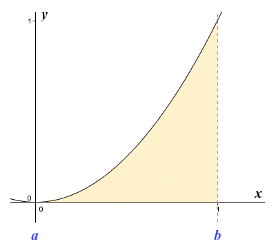
The graph of the function y = x 2 for 0 ≤ x ≤ 1
If we calculate the area of a triangle with a base one unit in length and a height of one unit, we get the result zero-point-five (0.5) units. This gives us a rough approximation for the area of the region under the graph. Of course, without knowing what the actual area is, it is difficult to say exactly how close our approximation is to the correct figure. In fact, the region under the graph has an area of exactly one third (1/3) of a unit. The calculations used to obtain this result will be described elsewhere in this section. For now, let's think about ways in which we could improve our estimate. We'll start by breaking the region under the curve down into rectangular strips. To start with, we'll use just four strips of equal width as shown below. Inside each strip, we construct a rectangle that has the same width as the strip. The height of each rectangle is such that the top left-hand corner of the rectangle just touches the graph.
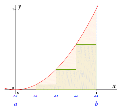
The area under the graph is divided into four equal strips
If we calculate the area of each rectangle and add the results together, we will have another estimate for the area of the region under the graph. To find the width of each strip, we divide the total width of the interval by the number of strips - in this case four. The width of an interval [a, b] is given by b - a, so the total width of the interval here is given by 1 - 0. We can think of each strip as a subinterval. The width of each subinterval represents an incremental change in x, which we represent as Δx. The symbol Δ is the Greek upper case letter Delta - the increment symbol. Putting all this together, the width of each subinterval can be expressed as:
| Δx = | 1 - 0 | = 1/4 |
| 4 |
The interval [0, 1] is thus divided into the following four subintervals:
[0, 1/4]
[1/4, 1/2]
[1/2, 3/4]
[3/4, 1]
Note that the height of the rectangles we have drawn is the same as the function value at the left end point of each rectangle (we could equally well have used the right-end point, but we have to start somewhere). Drawing our rectangles in this way means that we are carrying out what is called a left end point approximation. The endpoints of the subintervals are labeled (so that we can make reference to them) as follows:
x0 = 0
x1 = 1/4
x2 = 1/2
x3 = 3/4
x4 = 1
The next step is to calculate the function values at the left end point of each subinterval:
ƒ(x0 = 0 2 = 0
ƒ(x1) = (1/4) 2 = 1/16
ƒ(x2) = (1/2) 2 = 1/4
(x3) = (3/4) 2 = 9/16
We can bring all of this information together in a general mathematical formula that will enable us to calculate, and then add together (or sum), the areas of the rectangles in each subinterval. It will give us an approximation of the total area under the curve, which we'll call A (for area). We'll call the approximation itself L4 (to indicate that this is a left end point approximation using four rectangles). The only other label we need is an index (in the form of an integer subscript) to identify which subinterval we are talking about at any given point. We'll call this index i, and its value will range from i = 1 to i = 4 (because there are four subintervals). Here is the formula:
| A ≈ L4 = | 4 | ƒ(xi - 1) Δx = ƒ(x0) Δx + ƒ(x1) Δx + ƒ(x2) Δx + ƒ(x3) Δx |
| Σ | ||
| i = 1 |
| A ≈ L4 = | 0 × 1/4 + 1/16 × 1/4 + 1/4 × 1/4 + 9/16 × 1/4 |
| A ≈ L4 = | 7/32 = 0.21875 |
We use the Greek upper case letter Sigma (Σ) to signify that we are adding together (or summing) a series of terms. You may have encountered this kind of notation before. In case you haven't, some explanation of what's going on might be helpful. The number above the Sigma symbol, together with the expression underneath it, tells us that we are evaluating some function with respect to integer values of i, starting with i = 1 and ending with i = 4. The expression immediately following the Sigma symbol - ƒ(xi - 1) ∆x – tells us that each term in the sum is the product of ƒ(xi - 1) and Δx. In the first term of the sum, for example, the xi - 1 inside the function brackets refers to the value of x which we have labeled x0, because the initial value of i is one. The function is therefore evaluated for x = 0, and the result is multiplied by Δx, which is simply the width of each subinterval (1/4).
This new estimate is more accurate than the one we obtained using the triangle, even though there are some fairly big gaps between the top of the rectangles and the curve. Notice that, because we are using a left end point approximation with a function that is increasing, the estimate we get is an underestimate. This is because the rectangles never cover the entire area under the curve. For a function that is decreasing on an interval, a left end point approximation produces rectangles that cover all of the area under the curve, as shown in the illustration below. As you can see, they also cover areas that are not under the graph, so the estimate we get by summing the areas of the rectangles will be an overestimate.
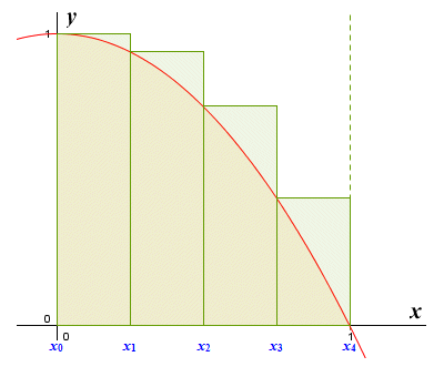
The graph of y = 1 - x 2 for 0 ≤ x ≤ 1
If we have a function that is both increasing and decreasing on an interval, then a left end point approximation will overestimate some parts of the area under the curve and underestimate others, as you can see below. Whether the approximation will be an overestimate or underestimate of the curve overall will of course depend on the function, and the interval in which we are interested.
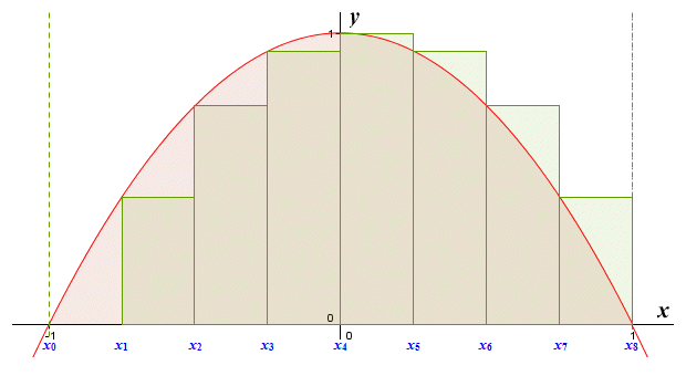
The graph of y = 1 - x 2 for -1 ≤ x ≤ 1
While we are on the subject of functions that both increase and decrease on an interval, let's think about how we handle functions that produce both positive and negative values over an interval, or that are negative over the whole interval. The simple answer is that for an interval (or part thereof) where the function is negative, we find the area of the region above the curve, in the same way that for an interval (or part thereof) where the function is positive, we find the area of the region below the curve. The principle is illustrated below.
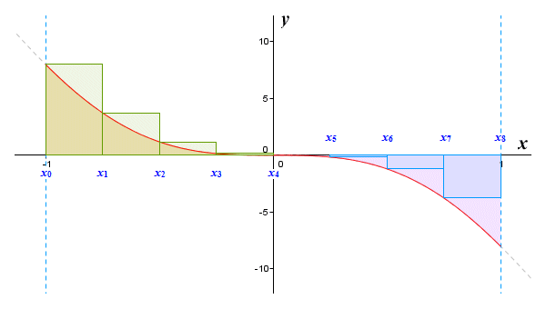
If the function is negative, we find the area above the curve
Since any region above the x axis is considered to be positive, and any region below the x axis is considered to be negative, then our approximation will be the total area of the rectangles above the x axis minus the total area of the rectangles below the x axis. In other words, the sum gives us the net value of the area between the graph and the x axis.
Let's do another approximation for the area under the graph of the function y = x 2, defined on the interval [0, 1]. This time, we'll use a right end point approximation.
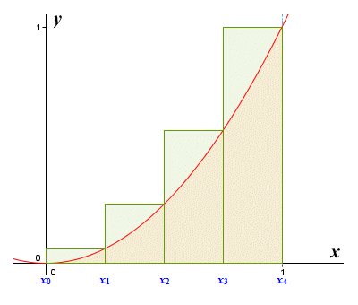
A right end point approximation with four subintervals
If we calculate the area of each rectangle and add the results together, we will have yet another estimate for the area of the region under the curve, but this time it will be an over estimate. The height of each rectangle this time around will be the same as the function value at the right end point of the rectangle. The endpoints of each subinterval have the same labels as they did previously, since the only thing that will change is the height of the rectangles. This time, though, we calculate the function values using the value of x at the right end point of each subinterval, as follows:
ƒ(x1) = (1/4) 2 = 1/16
ƒ(x2) = (1/2) 2 = 1/4
ƒ(x3) = (3/4) 2 = 9/16
ƒ(x4) = 1 2 = 1
We will call the approximation R4 to indicate that this is a right end point approximation using four rectangles. Once again, the approximation for the total area under the curve is given as the sum of the areas of the rectangles in each subinterval. We find the sum using the following formula:
| A ≈ R4 = | 4 | ƒ(xi) Δx = ƒ(x1) Δx + ƒ(x2) Δx + ƒ(x3) Δx + ƒ(x4) Δx |
| Σ | ||
| i = 1 |
| A ≈ L4 = | 1/16 × 1/4 + 1/4 × 1/4 + 9/16 × 1/4 + 1 × 1/4 |
| A ≈ L4 = | 15/32 = 0.46875 |
This estimate is again more accurate than the one we obtained using the triangle, but slightly less accurate than the left end point approximation. This is not altogether surprising, since there are some sizeable pieces of each rectangle that extend above the curve of the graph. Using a right end point approximation with a function that is increasing will always give us an overestimate, because the rectangles always cover the entire area under the curve plus some areas that are not under the graph. Interestingly, if we take the average of the left and right end point approximations, we get a figure that is not too far away from the actual area of the region under the graph:
| 0.21875 + 0.46875 | = 0.34375 |
| 2 |
Let's see what happens if we draw our rectangles so that their height is the same as the function value at the mid-point of each rectangle (we'll carry out what is called a mid-point approximation).
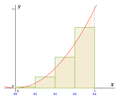
A mid-point approximation with four subintervals
We'll follow exactly the same procedure as before. We calculate the area of each rectangle, and add the results together to get an approximation for the area under the curve. We can still expect our approximation to be either an overestimate or an underestimate, but it remains to be seen which. This time, we will calculate the function values at the mid-point of each sub interval, as follows:
ƒ(x1m) = (1/8) 2 = 1/64
ƒ(x2m) = (3/8) 2 = 9/64
ƒ(x3m) = (5/8) 2 = 25/64
ƒ(x4m) = (7/8) 2 = 49/64
We'll call the approximation M4 to indicate that this is a midpoint approximation using four rectangles. As before, the approximation of the area under the curve is given as the sum of the areas of the rectangles in each subinterval. We find this sum using the following formula:
| A ≈ M4 = | 4 | ƒ(xim) Δx = ƒ(x1m) Δx + ƒ(x2m) Δx + ƒ(x3m) Δx + ƒ(x4m) Δx |
| Σ | ||
| i = 1 |
| A ≈ L4 = | 1/64 × 1/4 + 9/64 × 1/4 + 25/64 × 1/4 + 49/64 × 1/4 |
| A ≈ L4 = | 21/64 = 0.328125 |
This estimate is the most accurate so far. This will often be the case for functions that are reasonably well behaved. Nevertheless, there is still plenty of room for improvement. Before we move on, we should perhaps just briefly mention an alternative method for approximating the area under a graph called the trapezoid rule. Using this method, we still divide the interval into a number of subintervals of equal width, but instead of drawing a rectangle within each subinterval we draw a trapezoid (a trapezoid is a quadrilateral with two parallel sides) as shown below.
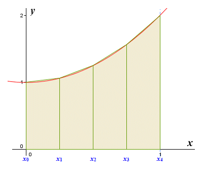
We can get an approximation of the area under the curve using trapezoids
The illustration shows the graph of the function y = x 2 + 1 for 0 ≤ x ≤ 1. The trapezoid approximation is more accurate than either the left end point approximation or the right endpoint approximation, because we can draw a trapezoid that matches the actual shape below the curve in each subinterval fairly closely. In fact, it turns out that using the trapezoid rule produces exactly the same result as taking the average of a left point approximation and a right point approximation for subintervals of the same width. This can be explained by the fact that the area of the trapezoid is equal to the average of the areas of the two corresponding rectangles.
None of the methods we have seen so far have given us a particularly accurate approximation. At this point, you may well be thinking that if we divide the area under the graph into a larger number of subintervals, we will get a more accurate approximation. If so, you are absolutely right. Using a greater number of subintervals means that the difference between the actual area under the graph in each subinterval and the area of the rectangle drawn within that subinterval will be smaller. This will improve the overall accuracy of our approximation. Let's see what a left end point approximation for the function y = x 2 for 0 ≤ x ≤ 1 looks like using eight sub intervals.
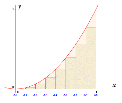
We can get a better approximation by using more subintervals
Without reproducing the entire calculation (which is starting to look somewhat cumbersome), we can report that adding up the areas of the rectangles gives us an approximation for the area under the graph of 0.2734375 - far more accurate than the result we got with only four subintervals, but still significantly less accurate than for the mid-point approximation. Even so, this is progress. It turns out that the more subintervals we have (regardless of whether we use the left end point, right end point, or mid-point approximation), the more accurate our approximation will be.
The methods described here for approximating the area of a shape whose area cannot be calculated using standard geometrical formulae is based on a method first used by the ancient Greeks, and which later became known as the method of exhaustion. The method involves finding the area of a shape by drawing a sequence of polygons (whose areas can be easily calculated) inside it. Eventually, the difference between the area of the shape and the total area occupied by the polygons will become so small that it can be ignored. Likewise, if we continue to divide the area under a graph into thinner and thinner rectangular slices, our approximation of the area under the graph will become increasingly accurate, but is this really practical? And how many calculations are we going to have to make? We'll come back to this question in due course.
The sums we have been calculating - by adding together the areas of the rectangles drawn in each subinterval - are called Riemann sums, after the German mathematician Georg Friedrich Bernhard Riemann (1826-1866). A Riemann sum is an approximation of the area of a region that is found by dividing the region into rectangles or trapezoids, calculating the area of each of these shapes, and then adding the results together. As we have seen, the accuracy of the approximation can be improved by dividing the region into smaller and smaller shapes, until the sum approaches what is known as the Riemann integral (we will be exploring the subject of integrals in detail elsewhere in this section).
The Riemann integral is essentially a number that is equal to the exact area of the region under the graph of a function, defined over some interval. This number falls between the results of two Riemann sums known as the upper and lower Riemann sums. The interval is divided into a number of subintervals of equal width, and a rectangle is drawn in each. The width of each rectangle will be the same as that of the subinterval.
In order to calculate the upper Riemann sum, the height of the rectangle in each subinterval must be set equal to the maximum value of the function over that subinterval, as illustrated below. The upper Riemann sum is the sum of the areas of these rectangles.
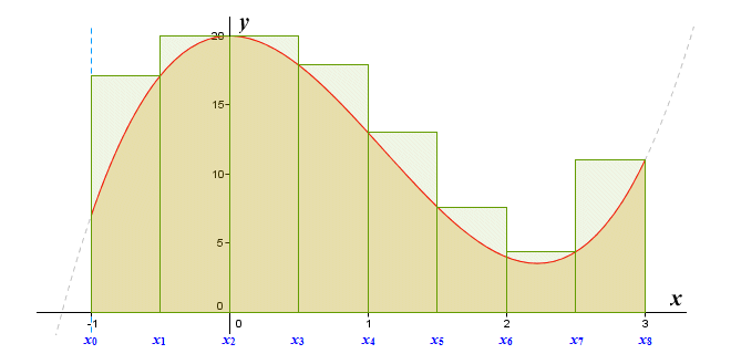
The rectangles effectively circumscribe the region under the graph
Suppose we have a function ƒ(x) defined on some interval that is divided into n equal subintervals. We can define the upper Riemann sum as:
| S = | n | υi (xi - xi - 1) |
| Σ | ||
| i = 1 |
where υi is the supremum (largest value) of ƒ(x) over the interval [xi - 1, xi].
In order to calculate the lower Riemann sum, the height of the rectangle in each subinterval must be set equal to the minimum value of the function over that subinterval, as illustrated below. The lower Riemann sum is the sum of the areas of these rectangles.
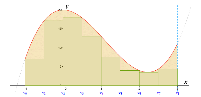
The rectangles are effectively inscribed within the region under the graph
We can define the lower Riemann sum as:
| S = | n | υi (xi - xi - 1) |
| Σ | ||
| i = 1 |
where υi is the infimum (smallest value) of ƒ(x) over the interval [xi - 1, xi].
Up to this point, we have been investigating the idea of approximating the area under the graph of a function defined on some interval by adding together the areas of a finite number of rectangles. If we want to find the exact area under the graph, we need to start thinking in terms of letting the number of rectangles approach infinity. This implies that the width (Δx) of the rectangles will approach zero. If this happens, both the upper and lower Riemann sums will converge to the same value, i.e. the Riemann integral - more often referred to as the definite integral. The good news is that we don't actually need to make an infinite number of calculations in order to calculate the definite integral, as we shall see.