| Author: | |
| Website: | |
| Page title: | |
| URL: | |
| Published: | |
| Last revised: | |
| Accessed: |
Line coding (also called digital baseband modulation or digital baseband transmission) is a process carried out by a transmitter that converts data, in the form of binary digits, into a baseband digital signal that will represent the data on a transmission line. The transmission line in question could be a link between two devices in a computer network, or it could form part of a much larger telecommunications network. The receiver is responsible for converting the incoming line-coded signal back into binary data.
There are many different line coding techniques, ranging in complexity from very basic unipolar schemes in which the presence or absence of a voltage is used to represent a binary one or a binary zero, to highly sophisticated multilevel schemes in which different signal amplitudes are used, each representing a unique grouping of binary digits.
The simplest line coding schemes are generally only used for relatively low-speed asynchronous transmission, in which data is sent in small independent blocks, and the receiver can re-synchronise itself with the transmitter at the start of each incoming block. For high speed synchronous applications in which much larger blocks of information are transmitted, timing becomes far more critical, as do factors such as noise and the potential presence in a signal of a net DC component.
The one thing that all line coding schemes have in common is that they modify signal levels in some way in order to represent digital data. In wired channels consisting of twisted-pair or coaxial cables, the line code manipulates voltage or current levels in order to generate electrical pulses that represent data values. In optical fibre channels, it represents the data values by modifying the intensity of pulses of light.
Line coding schemes can be broken down into five major categories:
The unipolar, polar and bipolar line coding schemes can be further categorised as either non-return to zero (NRZ) or return-to-zero (RZ) schemes. In a return-to zero scheme, if a signal uses a positive or negative voltage to represent a binary digit, the voltage must return to zero in the middle of the bit time. This has the advantage of providing the receiver with an opportunity to re-synchronise itself with the transmitter by using the additional transition as a clock signal. The down side is that it increases the complexity of both the line coding scheme and the circuitry needed to generate and decode it. It also effectively doubles the bandwidth required to transmit the signal.
We will be looking at the general characteristics each of the first three categories listed above (unipolar, polar and bipolar), after which we will look at some more specific examples of the line coding schemes in use today. We will also be looking at some of the techniques that can be used to prevent loss of synchronisation at the receiver and counter the build-up of a DC component in the transmitted signals. Before we do that, let's briefly consider some of the features we might expect to find in a modern line coding scheme. Most of the schemes in common use will demonstrate some or all of the following:
In a unipolar signaling scheme, all non-zero signalling elements have the same polarity - either they are all positive or they are all negative. It is analogous to a simple on-off keying scheme in which the presence of a voltage pulse signifies a binary one and the absence of a pulse signifies a binary zero. It is also the simplest kind of line-code we will encounter. The oldest unipolar line coding schemes are non-return-to-zero (NRZ) schemes in which the signal does not return to zero in the middle of the bit time. A positive voltage represents a binary one, and a zero voltage represents a binary zero.
An example of unipolar non-return-to-zero (NRZ) line coding
The advantages of unipolar NRZ are:
The disadvantages of unipolar NRZ are:
There is also a return-to-zero (RZ) version of unipolar line coding in which the logic high (binary one) signal voltage returns to zero half way through the bit time.
An example of unipolar return-to-zero (RZ) line coding
The advantages of unipolar RZ are:
The disadvantages of unipolar NRZ are:
In addition to their other disadvantages, neither unipolar NRZ nor unipolar RZ include any error detection or correction capability. Despite the fact that both schemes are easy to implement, they are therefore considered unsuitable for most real-world telecommunications applications.
Polar line coding schemes use both positive and negative voltage levels to represent binary values. Like the unipolar line coding schemes described above, polar signalling has both NRZ and RZ versions. For polar line coding, however, there are two different kinds of NRZ scheme. The first one we will look at is called NRZ-level (NRZ-L). Here, the voltage level determines the value of a bit. Typically, logic low (binary zero) is represented by a positive voltage while logic high (binary one) is represented by a negative voltage.
An example of polar NRZ-level (NRZ-L) line coding
The second polar NRZ line coding scheme we will look at is called NRZ-invert (NRZ-I). Here, the value of a bit is determined by the presence or absence of a transition from a positive voltage to a negative voltage, or vice versa. A transition signals that the next bit is a logic high (binary one), while no transition signals a logic low (binary zero). Note that in the illustration below, it is assumed that the line voltage was positive immediately before the start of the bit sequence. Because the first bit in the sequence is a binary zero, no transition occurs at the start of the sequence.
An example of polar NRZ-invert (NRZ-I) line coding
The advantages of polar NRZ are:
The disadvantages of polar NRZ are:
In addition to their other disadvantages, neither polar NRZ-L nor polar NRZ-I include any error detection or correction capability. A further potential problem arises with polar NRZ-L if there is a change of polarity in the system, in which case the signal logic gets inverted (zeros are interpreted as binary ones at the receiver, and vice versa). This problem does not arise with polar NRZ-I.
Polar NRZ-I is known as a differential code because it makes use of transitions rather than levels to signify logic values. This makes it less error prone in noisy environments, and eliminates the need for the receiver to determine polarity. A variant of polar NRZ-I is used to transfer data over a USB interface. In this variant, it is the transmission of a binary zero (as opposed to a binary one) that will trigger a transition.
USB uses bit-stuffing to force a transition whenever a long sequence of ones occurs. It does this by inserting a zero into the data stream after every sequence of six consecutive ones in order to trigger a transition. The stuffed bit is discarded by the receiver when it decodes the incoming signal. If the receiver detects that no transition has occurred after six consecutive ones have been received, it assumes that an error in transmission has occurred and discards the received data.
Polar RZ is the return-to-zero form of polar line coding. Some of the problems relating to polar NRZ line coding schemes are mitigated here through the use of three signalling levels. It is still the case that (typically) logic low is represented by a negative voltage and logic high is represented by a positive voltage, but in both cases the signal level returns to zero half way through the bit time and stays there until the next bit is transmitted (note that, somewhat confusingly, some sources refer to this line coding scheme as bipolar RZ, or BPRZ).
An example of polar RZ line coding
The advantages of polar RZ are:
The disadvantages of polar RZ are:
Like polar RZ, bipolar line coding schemes (sometimes called multi-level binary or duo-binary) use three voltage levels - positive, negative and zero. That, however, is pretty much where the similarity ends. Bipolar alternate mark inversion (AMI) uses alternate positive and negative voltages to represent logic high (binary one), and a zero voltage to represent logic low (binary zero). Although AMI is technically an NRZ line coding scheme itself, it was developed as an alternative to other NRZ schemes in which long runs of ones or zeros introduced a DC-component into the signal.
An example of bipolar AMI line coding
The advantages of bipolar AMI are:
The disadvantages of bipolar AMI are:
There is effectively no DC component - the signal is said to be DC-balanced - thanks to the use of alternating positive and negative voltage levels to represent logic high. This means that AC coupled transmission elements do not present any problems, and baseline wandering is unlikely to occur. The transition at the start of each binary one bit enables the receiver to maintain synchronisation, although long runs of zeros have the potential to be problematical. There is also the added advantage that polarity is not an issue, since both positive and negative voltages represent a logic high.
The pseudoternary version of bipolar line coding is essentially identical to AMI except that logic high is represented by a zero voltage and logic low is represented by alternate positive and negative voltages - the exact opposite of what happens with AMI.
An example of bipolar pseudoternary line coding
The advantages and disadvantages of pseudoternary line coding are the same as for AMI with the single exception that, rather than long sequences of zeros, it is long sequences of ones that can cause the receiver to lose synchronisation.
Manchester encoding is a widely used line coding scheme that embeds timing information in the transmitted signal. It does this by ensuring that there is a transition (high-to-low or low-to-high) in the middle of every bit time, making it easy for the receiver to retrieve a clock signal from the incoming bit stream and maintain synchronisation with the transmitted signal. The trade-off is a much higher bandwidth requirement than the other line coding schemes we have seen so far.
A logic high (binary one) is represented by a positive pulse with a period of half a bit time followed by a negative pulse of the same duration. Similarly, A logic low (binary zero) consists of a negative pulse followed by a positive pulse, each with a period of half a bit time. Essentially, the receiver looks for a transition in the middle of each bit time. A positive to negative transition is interpreted as a binary one, and a negative to positive transition is seen as a binary zero.
An example of Manchester line coding
Because each bit consists of both a positive and a negative pulse, Manchester encoding is sometimes referred to as bi-phase encoding. As you can see from the illustration, for each pair of consecutive zeros or consecutive ones, an additional transition is required at the boundary between the two bits to maintain the correct sequence of transitions.
There are similarities between Manchester encoding and both polar NRZ-L and polar RZ. Both polar NRZ-L and Manchester use two signal voltage levels, and both schemes feature a direct relationship between voltage state and logic state. The main difference is that polar NRZ-L uses a negative voltage to represent binary one and a positive voltage to represent binary zero, whereas Manchester uses a positive-to-negative transition to represent binary one and a negative-to-positive transition to represent binary zero.
Like polar RZ, Manchester encoding has a transition in the middle of every bit time. The main difference here is that, whereas the transitions in polar RZ all go from either positive or negative to zero volts, the transitions in Manchester go from positive to negative or from negative to positive. Note that there are actually two versions of Manchester encoding. The original scheme is as per the illustration above, and follows the convention first described by G. E. Thomas.
Thomas had graduated from Manchester University in 1948, and later became a member of staff there, and worked under Professor F. C. Williams on, among other things, the Manchester Mark 1 computer. Williams introduced Thomas to a phase modulation scheme, used for digital encoding, that was used to read and write data to and from the Manchester Mark 1's high-speed backing store. Thomas described the scheme, which we know today as Manchester encoding, in several papers, as well as in his PhD thesis "The design and construction of an electronic digital computer" (Manchester University, 1954).
The second version arises due to the fact that the Manchester signal is derived by XORing the binary data with the clock signal. Since the clock signal has two phases, two versions of Manchester encoding are possible, depending on which clock phase is used at the start of the line coding process.
The convention followed by a number of authors, and more importantly the convention specified by early Ethernet standards for 10 Mpbs transmission over coaxial and twisted pair cable, states that a logic low (binary zero) is represented by a positive to negative transition, and a logic high (binary one) is represented by a negative to positive transition. In other words, the exact opposite of the convention described by Thomas.
Manchester encoding (IEEE 802.3 version)
Manchester encoding addresses the shortcomings of polar NRZ-L and polar RZ schemes by ensuring that there is sufficient embedded timing information in the transmitted signal to enable the receiver to easily maintain synchronisation (there is at least one transition per bit time), and by eliminating the possibility of a DC component developing (each bit spends half its duration at a positive voltage level and the other half at a negative voltage level), which also removes the possibility of baseline wandering. The main disadvantage of Manchester encoding, and the main reason it is not used for Fast Ethernet (100 Mbps) and above, is because of its inefficient use of bandwidth.
Manchester encoding suffers from the problem that, if the signal gets inverted (i.e. changes polarity) whilst in transit, it is transformed from one convention to the other, leading to polar ambiguity (the receiver will interpret ones as zeros, and vice versa). The problem can be overcome by using a variant of Manchester encoding called differential Manchester encoding. Whereas Manchester encoding could be described as combining aspects of polar RZ and NRZ-L, differential Manchester is more like a combination of RZ and NRZ-I.
There is still a transition in the middle of each bit time, but there is only a transition at the start of a bit time if the bit will be a logic high (binary one). There is no transition at the start of the bit time if the bit will be a logic low (binary zero). It is the presence or absence of a transition at the beginning of a bit time that signifies what logic state the bit represents. Neither the direction of the transition nor the actual voltage level on the line during the bit time have any significance in this respect. This means, effectively, that if the signal gets inverted, it still represents the same bit pattern.
Differential Manchester encoding
Differential Manchester encoding addresses the problems associated with NRZ-I coding, and essentially has the same advantages and disadvantages as Manchester encoding. There is no DC component in the signal, baseline wandering is not a problem, and the embedded timing engendered by the presence of at least one transition per bit time ensures that the receiver can maintain synchronisation. There is also the added advantage that if the signal is inverted somewhere along the transmission path, the information carried by the line-coded signal will not change.
Unfortunately, differential Manchester suffers from the same inefficiency as Manchester in terms of bandwidth usage, but it has seen commercial use (it was used, for example, in IEEE 802.5 token ring local area networks). An important feature of differential Manchester is that, like polar NRZ-I, it is a differential line coding scheme, relying solely on the presence or absence of transitions at the start of each bit time to signal the logic state of each bit. This is an advantage because it is easier for a receiver to detect the occurrent of a voltage transition (regardless of direction) than to measure a voltage level against a threshold, or to determine the direction of a transition, in a noisy environment.
Manchester and differential Manchester are DC-balanced line coding schemes that provide ample embedded timing information, but they don't make efficient use of the available bandwidth. This is not a huge problem for environments like Ethernet LANs, because bandwidth limitations are not usually an issue. Both the number of users on the network and the types of applications they use are known, enabling network administrators to calculate the network's bandwidth requirements and ensure that the network has sufficient capacity to cope with demand.
The rise of the Internet, however, has created an environment in which the demand for bandwidth has grown exponentially. Making efficient use of bandwidth is therefore a critical factor in ensuring that networks maintain sufficient capacity to cope with demand. And, whilst the Internet and the telephone network are - at least for the time being - still two very different kinds of network, voice and data traffic is often transmitted simultaneously over the same network infrastructure. The systems carrying that traffic must therefore exhibit a high degree of bandwidth efficiency.
In North America, from the early 1960s onwards the trunk networks connecting telephone exchanges were implemented using carrier systems developed by AT&T Bell Laboratories for the digital transmission of multiplexed telephone calls. These carrier systems were called T-carriers, and a hierarchy of five different levels was originally proposed, with each level corresponding to a different data-carrying capacity.
At the lowest level, the T1 carrier has a gross bit rate of 1.544 Mbps and can carry 24 telephone calls simultaneously over a copper-wire cable comprising two twisted-pairs. The only other T-carrier to actually see widespread use is the T3 carrier, which consists of 28 multiplexed T1 channels, has a gross bit-rate of 44.736 Mbps, and can carry up to 672 calls simultaneously.
In Europe, a similar E-carrier system was developed to fulfil essentially the same role as the North American T-carrier system. The E-carrier system, which was subsequently adopted by most other countries in the world (with the exception of Japan), is not directly compatible with the T-carrier system. At the lowest level in the E-carrier system, for example, an E1 carrier has a gross bit rate of 2.048 Mbps and can carry 32 simultaneous phone calls. The one thing both systems have in common, however, is that they both use modified versions of alternate mark inversion (AMI), because it makes efficient use of bandwidth and is DC-balanced.
The problem with unmodified AMI, as you may recall, is that whereas binary ones are coded as alternating negative and positive pulses, binary zeros are always coded using the absence of a pulse. Long sequences of binary zeros can cause the receiver to lose synchronisation because there are no transitions. The solution is to break these sequences up by replacing them with an alternative bit pattern that does contain transitions, enabling the receiver to maintain synchronisation. The replacement bit pattern is subsequently converted back into the original sequence of binary zeros.
The T-carrier system uses line coding schemes such as bipolar 8-zero substitution (B8ZS), a form of AMI in which sequences of 8 zeros are replaced with a substitute bit pattern containing both ones and zeros. The E-carrier system uses a similar line coding scheme called high density bipolar order 3 (HDB3), also a modified form of AMI, in which runs of 4 binary zeros are replaced with an alternate bit pattern. We'll take a closer look at HDB3 to give you a better idea of how run-length limited encoding schemes work in general.
In HDB3, which is used at all levels of the E-carrier system, any run of 4 consecutive binary zeros will be replaced by one of four possible substitute bit patterns, depending on whether the most recent binary one was transmitted as a positive or a negative pulse, and on whether the number of pulses transmitted since the most recent HDB3 substitution is odd or even. This probably sounds more complicated than it actually is. We can break down the way in which the way in which the correct substitute bit pattern is chosen using the following table:
| Polarity of previous pulse |
Odd number of pulses since last substitution |
Even number of pulses since last substitution |
|---|---|---|
| Negative | 0 0 0 - | + 0 0 + |
| Positive | 0 0 0 + | - 0 0 - |
The following illustration shows how a typical bit sequence containing runs of four or more zeros would be coded. Note that, for the purposes of this exercise, we are assuming that either there have been no substitutions before the start of the sequence, or that the number of pulses transmitted before the sequence started was an even number.
An example of high-density bipolar order 3 (HDB3) coding
The most important point to note here is that the receiver will recognise the substitution for what it is because any pulses transmitted in the replacement sequence will be code violations - they will break the rule that a positive pulse must be followed by a negative pulse, and vice versa.
MLT-3 (multi-level transmit) is, like polar NRZ-I and differential Manchester, a differential line coding scheme. The "3" in the name reflects the fact that, whereas both of the aforementioned schemes use only two signal levels (positive and negative) to represent binary values, MLT-3 uses three levels (positive, negative and zero). It is also classed as a multi-level encoding scheme, because it uses more than two levels to represent binary data.
On that basis, we could probably also describe polar RZ, bipolar AMI and pseudoternary encoding as multi-level schemes. The difference is that, in polar RZ, the zero signal level is not used to represent a logic value, and in bipolar schemes, the absence of a pulse always represents a binary zero while the presence of a pulse (positive or negative) always represents a binary one. In MLT-3, not only are all three signal levels used to represent data, but each signal level can represent a different logic value, depending on the signal level and the logic value of the preceding bit.
The rules are basically as follows:
MLT-3 cycles through the voltage levels sequentially (from negative to zero to positive to zero), moving to the next state to signal a binary one or maintaining its current state to signal a binary zero. The illustration below shows how a typical bit pattern would be encoded using MLT-3. Note that, for the purposes of this exercise, we are assuming that the most recent non-zero signal level prior to the start of the sequence was negative.
MLT-3 encoding of a typical bit sequence
Because transitions only occur when a logic high is to be transmitted, MLT-3 has a relatively low bandwidth requirement. The worst-case scenario from a bandwidth perspective would be a long sequence of binary ones, which would cause the signal to make one complete cycle (+0-0 or -0+0) in the space of four bits, as shown below. MLT-3 thus requires less bandwidth than most other binary (two-level) or ternary (three-level) line coding schemes that have the same bit rate.
Runs of binary ones increase the average bandwidth requirement
Because MLT-3 requires four transitions to complete one complete cycle, the maximum fundamental frequency that must be supported by the transmission medium is only one quarter of the baud rate, making MLT-3 suitable for transmission over twisted-pair copper wire cables. Consequently, MLT-3 has been used successfully for 100BASE-TX Ethernet, the predominant form of Fast Ethernet (100 Mbps), operating over two wire pairs in category 5 (or above) twisted pair cables.
As you may have surmised from the MLT-3 signalling diagrams above, MLT-3 is not a DC-balanced line coding scheme. It is also susceptible to loss of synchronisation at the receiver if there are long runs of zeros. One solution to this problem is to use block coding. The data to be transmitted is broken down into fixed-length blocks. Each block is replaced, prior to transmission, with a slightly longer block selected from an encoding table. The replacement block contains a unique bit pattern designed to ensure that the transmitted signal will contain a minimum number of transitions, ensuring that the resulting line code is DC-balanced and that the receiver can remain synchronised.
The block coding scheme used with MLT-3 and Fast Ethernet is called 4B5B. The binary data is broken down into blocks of four bits. Four bits gives us 16 possible bit sequences (2 4), so we need 16 different codes to represent the data. In 4B5B, each 4-bit block of data is replaced with a unique 5-bit code. Five bits produces 32 unique bit patterns (2 5), from which 16 have been selected to represent the data. Each of the 5-bit codes used will produce at least two transitions in the output signal. The following table lists the 4-bit data sequences, together with the 5-bit codes used to represent them.
| Data | Code | Data | Code |
|---|---|---|---|
| 0000 | 11110 | 1000 | 10010 |
| 0001 | 01001 | 1001 | 10011 |
| 0010 | 10100 | 1010 | 10110 |
| 0011 | 10101 | 1011 | 10111 |
| 0100 | 01010 | 1100 | 11010 |
| 0101 | 01011 | 1101 | 11011 |
| 0110 | 01110 | 1110 | 11100 |
| 0111 | 01111 | 1111 | 11101 |
The presence of the extra bit in each code effectively means an additional 25% bandwidth requirement. Even so, the use of 4B5B with MLT-3 still results in a highly efficient use of bandwidth by comparison with line coding schemes like Manchester encoding. The main downside of the use of block coding with a differential line coding scheme like MLT-3 is increased complexity, requiring more sophisticated electronic circuitry to handle the encoding and decoding.
The 2B1Q (two binary, one quaternary) line coding scheme is the first of three very different multi-level schemes we will be looking at. The idea behind multi-level schemes generally is to encode more than one data bit per signal symbol in order to maximise bandwidth efficiency. Putting this more formally, the aim is to encode m data elements per signal element using n signal elements. This is often reflected in the name given to a particular line coding scheme. In 2B1Q, for example, each dibit (dibit is the name given to a pair of bits) is represented by one quaternary symbol.
There are four quaternary symbols in 2B1Q (the word quaternary means "consisting of four units or members"). Each quaternary symbol is represented by one of four different signal levels. 2B1Q is thus a four-level pulse amplitude modulation (PAM-4) scheme, so called because the information is encoded in the amplitude of the signal pulses. There are two positive and two negative signal levels, with equal spacing between adjacent levels. The illustration below shows what a typical 2B1Q signal looks like.
2B1Q is a four-level pulse amplitude modulation scheme
Typical signal levels in a 2B1Q transmission are +450 millivolts, +150 millivolts, -150 millivolts and -450 millivolts, which gives an even spacing of 300 millivolts between levels. In the illustration above, we have used the numbers +3, +1, -1 and -3 to represent pulse levels rather than actual voltages. The table below pairs each dibit with the pulse level used to represent it.
| Data | Output |
|---|---|
| 00 | -3 |
| 01 | -1 |
| 10 | +3 |
| 11 | +1 |
The values in this table are easy to derive. The pulse level chosen to represent each dibit depend on the bit values. The value of the first bit determines polarity: if the first bit is zero, the output is negative; if the first bit is one, the output is positive. The value of the second bit determines the magnitude of the output: if the second bit is zero, the output has a magnitude of 3; if the second bit is one, the output has a magnitude of 1.
2B1Q is one of the line coding schemes used to transmit data over an Integrated Services Digital Network (ISDN) Basic Rate Interface (BRI). That's the part of an ISDN network that connects an exchange terminator (ET) in a local telephone exchange to a network terminator (NT1 or NT2) at the customer's premises for ISDN's basic rate service. This part of the network is sometimes called the U loop, or U interface.
Because 2B1Q encodes two bits of data per signal symbol and does not include any redundant data in the line code, it makes very efficient use of bandwidth. The down side is that 2B1Q is not DC-balanced. Long runs of dibits with the same bit values can introduce a significant DC component into the signal, and will also result in the absence of transitions in the signal, potentially causing loss of synchronisation.
The next multi-level line coding scheme we want to look at is 8B6T (eight binary, six ternary), which can also be classed as a multi-level scheme despite the fact that it uses only three signalling levels (positive, negative and zero). 8B6T is a rather unusual coding scheme that uses three-level pulse amplitude modulation (PAM-3) to code a block of eight binary digits onto a sequence of six signalling elements. Each signal element takes one of three values - positive, negative, or zero. The signalling elements in 8B6T are thus said to be ternary symbols (from the Latin word ternarius, which means "composed of three items").
A sequence of eight binary digits has only 256 possible permutations (2 8 = 256), whereas there are 729 unique ways in which in which six ternary signal levels can be combined (3 6 = 729). This leaves 473 redundant signalling combinations that can be used to provide synchronisation and error detection capabilities, as well as ensuring that the signal output is balanced with respect to DC (we'll see how that works shortly). The illustration below shows how a typical sequence of bits would be encoded using 8B6T.
8B6T maps eight bits onto six signal symbols
The diagram shows three groups of six signal elements. Each group encodes an eight-bit binary number, which can also be represented as a two-digit hexadecimal number. Unlike 2B1Q, 8B6T does not have a simple rule-based method for deriving the signal pattern to be used to represent each eight-digit bit pattern. Instead, a lookup table must be used. The look-up table maps each 8-digit binary number to the appropriate signal pattern. Part of a hard-copy version of the look-up table, available on McGraw Hill's Access Engineering website, is shown below.
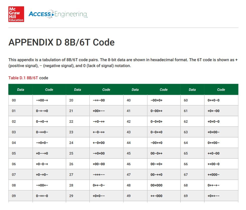
Part of the 8B6T look-up table
Each signal pattern in the lookup table has a weighting of either 0 or +1. In other words, there will either be the same number of positive or negative pulses (weighting = 0), or there will be one more positive pulse than there are negative pulses (weighting = +1). None of the signal patterns in the table have a weighting of -1. This obviously has the potential to create a significant DC component in the output signal, because the number of positive pulses will quickly become significantly larger than the number of negative pulses.
What actually happens is that the transmitter circuitry keeps track of the weighting on the line, which is initialised to zero before transmission begins. Any signal pattern with a weighting of 0 will be transmitted unchanged. The first signal pattern with a weighting of +1 will also be transmitted without change, but the line weighting will be set to +1. The next signal pattern to have a weighting of +1 is inverted, giving it weighting of -1, before it is transmitted. The balance having been restored, the line weighting is set back to 0, and remains there until the next signal pattern with a weighting of +1 is encountered.
In the above example, all three of the signal patterns matching the three binary octets originally had a weighting of +1. The second signal pattern (highlighted) has therefore been inverted to give it a weighting of -1. An inverted signal pattern is recognised as such by the receiver because of its negative weighting (the inverted signal patterns belong to the set of redundant signalling combinations we mentioned earlier). The receiver knows that the signal pattern has been inverted, and reverses the process prior to decoding.
In addition to 8B6T's bandwidth efficiency, the frequent transitions in the signal enable the receiver to maintain synchronisation, and the use of pre-defined signal patterns facilitates a degree of error detection. It might be tempting to think of 8B6T as a block coding scheme like 4B5B (see above). The difference is that 4B5B replaces each 4-bit block of data with a 5-bit code taken from its encoding table, and the data is then transmitted using a line coding scheme such as MLT-3. The 8B6T encoded data is transmitted without any additional encoding. It can thus be considered to be a line coding scheme in its own right. 8B6T is the line coding used for Ethernet 100BASE-T4, which was an early implementation of Fast Ethernet.
The last multi-level line coding scheme we are going to look at is 4D-PAM5 (four-dimensional five-level pulse amplitude modulation). As the rather long-winded name suggests, 4D-PAM5 uses five signalling levels (we'll refer to them as -2, -1, 0, 1 and 2). The 4D part refers to the fact that data is transmitted using four wire pairs simultaneously. Before we talk about 4D-PAM5 in more detail however, a little background information might help to put things into context.
1998 saw the emergence of Gigabit Ethernet, which has a gross bit rate of 1 Gbps (1000 Mbps) - a tenfold increase in performance over Fast Ethernet. The IEEE 802.3z 1000Base-X standard supports three media types: 1000Base-SX operates over multi-mode optical fibre; 1000Base-LX operates over single and multi-mode optical fibre; and 1000Base-CX operates over short-haul shielded twisted pair cable (cable segments are limited to a maximum length of 25 metres).
The real challenge was seen as getting Gigabit Ethernet to work over existing category 5 (or higher) unshielded twisted pair cables. This would enable Gigabit data rates to be achieved using the installed cable infrastructure, eliminating the need to rip out and replace existing cable plant. The result of extensive research and development efforts bore fruit in 1999, with the release of the IEEE 802.3ab 1000BASE-T standard.
The success of Fast Ethernet had already shown that bit rates of 100 Mbps could be achieved over a single twisted pair cable. The predominant form of Fast Ethernet is IEEE 802.3u 100BASE-TX, which runs over two wire pairs in a category 5 (or above) twisted-pair cable. One pair of wires is used for each direction, providing full-duplex operation.
The thing about twisted-pair Ethernet cables is that they actually consist of four wire pairs. 1000BASE-T Gigabit Ethernet uses all four pairs, which obviously has the potential to double the throughput. But that is just the beginning of the story. A category 5 cable that meets all of the required standards can support frequencies of up to 125 MHz.
As we saw earlier, the MLT-3 line coding scheme used for 100BASE-TX is not DC-balanced, and does not guarantee the presence of sufficient transitions to enable the receiver to maintain synchronisation. The data is therefore encoded before transmission using the 4B5B block coding scheme, which maps four data bits onto a 5-bit code. That explains why the actual gross data rate is only 100 Mbps, despite the fact that the 125 MHz analogue bandwidth allows a signalling rate of 125 megabaud.
The 4D-PAM5 line coding scheme uses five different signalling levels and transmits on all four wire pairs simultaneously, achieving a baud rate of 125 megabauds per second on each channel, and an overall baud rate of 500 megabauds per second. Every symbol transmitted corresponds to two bits of data, so the gross bit rate is 1,000 Mbps - 8 bits during each 8- nanosecond cycle. The diagram below compares typical 100BASE-TX MLT-3 and 1000BASE-T 4D-PAM5 signals (note that we have only shown one of the four 4D-PAM5 channels).
4D-PAM5 line coding has the same baud rate as MLT-3 but uses 5 signalling levels
MLT-3 transmits one signal symbol per clock cycle, although the use of 4B5B block coding with MLT-3 means that each signal symbol only encodes 4/ 5 data bits. 4D-PAM5 encodes two data bits per symbol on each channel, enabling the transmission of eight data bits per clock cycle. The number of unique signalling patterns required to represent every possible 8-bit data word is 2 8 = 256. However, with four channels and five signalling levels to choose from, it is possible to generate 5 4 = 625 unique signal patterns. As a result, the 4D-PAM5 line coding scheme has considerable redundancy.
What's even more remarkable is the fact that, whereas MLT-3 uses two wire pairs to achieve full-duplex 100 Mbps operation, 4D-PAM5 uses a single wire pair to achieve full-duplex operation at a gross bit rate of 250 Mbps. In other words, data is transmitted in both directions simultaneously over a single wire pair at a gross bit rate of 250 million bits per second! It probably comes as no surprise to learn that this two-way flow of traffic results in a huge number of collisions on the wire pairs, resulting in some extremely complex voltage patterns.
1000BASE-TX implements full-duplex operation over four wire pairs
In order to ensure that the transmitted signal can be correctly interpreted by the receiver, the input data is "scrambled" using pseudo-random values in order to spread the transmitted power as evenly as possible over the frequency spectrum. The output from the scrambler is encoded using a convolutional code - essentially a special kind of block coding. The kind of convolutional code used is sometimes called a trellis code because the diagrams used to represent the encoding patterns look a bit like a garden trellis.
The encoding process adds a redundant bit to the data to be transmitted so that the receiver can recover the data even if some errors are introduced during transmission - this is known as forward error correction (FEC). This is possible because, as we mentioned above, with four channels and five signalling levels available, there are 625 possible signalling patterns. We can represent every possible 9-bit code word with just 512 signalling patterns (2 9 = 512). This provides 100% redundancy in terms of data representation and still leaves 113 signalling patterns that can be used to transmit Ethernet control codes.
The code words used to represent the data are chosen by the trellis encoding process in order to minimise the possibility of a DC component developing in the transmitted signal, and to maximise the ability of the receiver to maintain synchronisation and correctly decode the incoming signal (the subject of convolutional coding, including trellis coding, will be dealt with in more depth in a separate article).
The complex electronic circuitry in each node that encodes the outgoing signal and decodes the incoming signal on each wire pair is combined into a single hybrid encoder/decoder unit. These hybrid units use an array of sophisticated signal processing techniques, including pulse shaping, echo cancellation and adaptive equalisation, in order to counter the effects of noise, echo and crosstalk, and to separate the incoming signals from the outgoing signals (a discussion of how such techniques work is somewhat outside the scope of this article but we will be looking at them in more detail elsewhere).