| Author: | |
| Website: | |
| Page title: | |
| URL: | |
| Published: | |
| Last revised: | |
| Accessed: |
Rolle's theorem is named after the French mathematician Michel Rolle (1652-1719). The theorem essentially makes a statement about a non-constant function that is both continuous and differentiable over some defined interval, and for which the function returns the same value at each end of the interval. Remember that if a function is continuous, it has no gaps or breaks. In other words, you can draw a graph of the function by hand without taking your pencil off the paper. A function is differentiable if it changes smoothly, with no sudden changes in direction (in other words, you must be able to draw a tangent at any point within the interval). Suppose we have a function ƒ(x) that is continuous on some interval [a, b]. The function will take the same value at each end of the interval. In other words, ƒ(a) is equal to ƒ(b). Rolle's theorem states that there must be at least one point c between a and b at which the function changes direction. The principle is illustrated below.

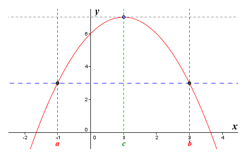
The graph of the function ƒ(x) = -x 2 + 2x + 6
The illustration shows the graph of the function ƒ(x) = -x 2 + 2x + 6 defined on the interval [a, b], where a is equal to minus one (-1), and b is equal to three (3). The values taken by the function at a and b will be:
ƒ(a) = -a 2 + 2a + 6 = -1 + (-2) + 6 = 3
and
ƒ(b) = -b 2 + 2b + 6 = -9 + 6 + 6 = 3
The interval [a, b] satisfies the requirements of Rolle's theorem, since the function is continuous and differentiable at all points between a and b, and because the values of ƒ(a) and ƒ(b) are equal. There must therefore be at least one point c within the interval for which a < c < b, and at which the function changes direction. From the illustration above, we can clearly see that this is the case. The function increases in value until it reaches its maximum value at point c, where x is equal to one (1). It then starts to decrease in value once more. Since we know that the function changes direction at point c, then by definition it must be a stationary point.
A stationary point is a special kind of critical point on the graph of a function at which the derivative (i.e. the slope of the graph) is zero (0). The tangent to the graph at such a point is parallel to the x axis. For an interval [a, b] that satisfies the requirements of Rolle's theorem, it will also be parallel to the line that intercepts points ƒ(a) and ƒ(b). In the illustration above, the tangent to the point ƒ(c) is shown as a dashed grey line, while the line that intercepts points ƒ(a) and ƒ(b) is shown as a dashed blue line. You can see that the lines are parallel both to each other and to the x axis.
Stating Rolle's theorem a little more formally, if a real-valued function ƒ(x) is continuous on a closed interval [a, b], is differentiable on the open interval (a, b), and ƒ(a) = ƒ(b), there must exist a point c within the open interval (a, b) such that a < c < b and:
| d | (ƒ(c)) = 0 |
| dx |
or (using Lagrange notation):
ƒ′(c) = 0
Like the intermediate value theorem, Rolle's theorem essentially just tells us something that we can grasp intuitively by looking at any graph that satisfies the necessary criteria. In this case, we are interested in any continuous and differentiable function, defined on an interval [a, b], where the function has the same value at each end of the interval. The theorem tells us that the function will change direction at least once. What it doesn't tell us is where the change of direction will occur, or even how often the function will change direction within the interval - just that it will change direction at least once, somewhere within the interval.
Although the principles underlying Rolle's theorem had probably been understood for centuries, as far as is known Rolle was the first mathematician to offer a formal proof for the theorem, which he published in 1691. Although Rolle's theorem is of no great significance when considered in isolation, it is in fact a special case of the mean value theorem, which is arguably one of the most important theoretical tools in calculus. We will be looking at the mean value theorem in some depth in a separate page.